Prediction of binding hot spot residues by using structural and evolutionary parameters

Prediction of binding hot spot residues by using structural and evolutionary

parameters

Roberto Hiroshi Higa

and Clésio Luis Tozzi

Departamento de Engenharia de Computação e Automação Industrial, Faculdade de Engenharia Elétrica e

de Computação, Universidade Estadual de Campinas, Campinas, SP, Brazil.

2

_{Embrapa Informática Agropecuária, Empresa Brasileira de Pesquisa Agropecuária, Campinas, SP, Brazil.}

Abstract

In this work, we present a method for predicting hot spot residues by using a set of structural and evolutionary param-eters. Unlike previous studies, we use a set of parameters which do not depend on the structure of the protein in com-plex, so that the predictor can also be used when the interface region is unknown. Despite the fact that no information concerning proteins in complex is used for prediction, the application of the method to a compiled dataset described in the literature achieved a performance of 60.4%, as measured by F-Measure, corresponding to a recall of 78.1% and a precision of 49.5%. This result is higher than those reported by previous studies using the same data set.

Key words:hot spots prediction, protein structure, hot spots. Received: December 23, 2008; Accepted: May 6, 2009.

Introduction

Protein-protein interactions play a key role in most biological processes and are of great importance for living cells. Although the principles governing this process are still not fully understood, it is well-known that binding en-ergy is not evenly distributed among interface residues, with a large contribution coming from only a small subset (Moreira et al., 2007). These residues are referred to as binding hot spots.

Recent interest in this protein-protein interface as drug targets (Arkin and Wells, 2004) has highlighted the importance of identifying hot spots systematically. Usually, this is done through site-directed mutagenesis ex-periments such as the alanine scanning technique (DeLano, 2002). These experiments aim to evaluate the impact in terms of free energy of binding caused by mutations to alanine of specific interface residues. This, however, can demand a significant experimental effort. In this scenario, there is growing interest in cheaper and faster computa-tional hot spot prediction, as they could help biologists fo-cus their experimental efforts only on those interface residues that present the best chance of being hot spots.

Most methods for predicting hot spots rely on physi-cal models to evaluate the impact in terms of free energy of binding due to specific site mutations inside the interface region (Kortemme and Baker, 2002). On the other hand,

structure-based methods try to discriminate hot spots from the rest of the interface residues by analyzing their differ-ences through a set of structural and chemical properties. Bogan and Thorn (1998) reported that hot spot residues tend to form clusters near the center of the interface, and are characterized as polar residues protected by a ring of hydro-phobic ones that form a structure they call an O-ring. They also analyzed the amino acid preference for being a hot spot and found tryptophan, tyrosine and arginine as those presenting the highest propensities. Another property com-monly used for characterizing hot spots is residue conser-vation. Hot spots have been characterized both as sequen-tially conserved polar residues (Hu et al., 2000) and as structurally conserved ones (Ma et al., 2003). Li et al.

(2004) also analyzed the geometric organization of struc-turally conserved residues concluding that most of hot spots are found in regions characterized by a pocket well-complemented by protruding residues. Other methods in-clude those from Guneyet al.(2008) that predict hot spots using residue conservation and solvent accessible surface areas - ASA, and the one from Banet al.(2006) that applies a geometric method to predict hot spots by detecting resi-dues located on regions of the interface protected from the periphery.

Only recently, Darnellet al.(2007) approached this problem using discriminant analysis, compiling a high quality and non-redundant data set containing interface res-idues with both types of information: structure and site di-rected mutagenesis. The best predictor they found involved both structural, chemical and energetic parameters and a

www.sbg.org.br

Send correspondence to Roberto Hiroshi Higa. Av. André Tosello 209, Caixa Postal 6041, 13086-886 Campinas, São Paulo, Brazil. E-mail: roberto@cnptia.embrapa.br.

combination of classifiers using a simple OR rule. It achieved a performance of 55%, as measured by F-Mea-sure, corresponding to a recall of 72% and a precision of 44%. Using the same data set and a different strategy for combining classifiers, Higa and Tozzi (2008) achieved a slightly higher performance, corresponding to an F-Mea-sure of 56.5%.

In this work we present a method for predicting hot spot residues which rely on a set of structural and evolu-tionary parameters. Unlike those used by all previously proposed methods, this set of parameters does not depend on the knowledge of protein structure in complex. An SVM classifier (Cristianini and Shawe-Taylor, 2000) with thea posterioriprobability estimated according to Plat’s method (Platt, 2000) and implemented in SVMLib (Chang and Lin, 2001) is used for prediction. Despite the fact that no infor-mation concerning proteins in complex is used, the method achieved a performance of 60.4%, measured by F-Measure, corresponding to a Recall of 78.1% and a Precision of 49.5%, which is higher than those previously obtained us-ing the same data set.

Material and Methods

Dataset

We used the data set compiled by Darnell et al.

(2007). Considering that the number of proteprotein in-terfaces with organized information characterizing them both structurally and energetically is quite limited, this data set constitutes the most representative one compiled for an-alyzing hot spot residues. It is composed of interface resi-dues experimentally mutated to alanine and having a re-ported free energy of binding (DDG) in the AseDB database (Bogan and Thorn, 1998) or in a data set from Kortemme and Baker (2002). The criterion used to define an interface residue is the presence of at least one atom within 4 Å of an atom of the interacting protein. In addition, only proteins whose crystal structure presented a resolution inferior to 3 Å and sequence identity to any other sequence in the data set lower than 35% were considered.

Moreover, we removed from the original data set those residues for which we could not calculate the sponding conservation property (see below). This corre-sponds to 15 residues. So, we effectively used a data set containing 233 residues, 24% of them corresponding to hot spot residues. Each residue in the data set was labeled a hot spot if its corresponding DDG reported in AseDB was higher or equal to 2.0 kcal/mol. Otherwise, it was labeled a non-hot spot residue.

Structural and evolutionary parameters

A set of 43 evolutionary and structural parameters, presented below, were used to characterize an interface res-idue. Note that all of them are calculated using only the structure of the protein that the residue belongs to.

• Amino acid type (x1, x2): we used two indexes

(Hagertyet al., 1999), derived from the Aaindex database (Kideraet al., 1985), to represent the 20 standard amino acid types. These two indexes sum-marize a collection of more than 400 indexes de-scribing biochemical properties for each of the 20 standard amino acids. Unlike the equidistant 20-bit code commonly used to encode amino acid type, the more similar two amino acids are, the closer they are in the space defined by (x1, x2). In

particu-lar, the two indexes that we used are strongly corre-lated to residue size and hydrophobicity on one hand and to residue preference for being in a loop or strand on the other (Hagertyet al., 1999). • Evolutionary profile (x3,..., x22): first we used the

software Blast (Altschulet al., 1997). As parame-ters, we used substitution matrix BLOSUM62 and expect value = 0.1, against the Swissprot/Uniprot knowledgebase release 9.6 (Apweileret al, 2004) in order to find similar protein sequences. Then, se-quences in the blast result were filtered according to HSSP threshold (Rost, 1999) to keep only homo-logue sequences. Two protein sequences in the original data set (Darnellet al., 2007) did not sur-vive this filtering process (at least five homologue sequences). Consequently, in our experiment only 233 interface residues were considered. After that, we used the software ClustalW (Higgins et al., 1994), with substitution matrix series BLOSUM, gapopen = 3.0 and gap ext = 0.1, using the resulting set of homologue sequences to build the final mul-tiple sequence alignment (MSA). Each member of the profile corresponds to the percentage of the amino acid type present in the MSA.

• Conservation score (x23): the residue conservation

score was calculated using the same MSA used for extracting the evolutionary profile parameters. The residue conservation score corresponds to evolu-tionary pressure, calculated by using the software rate4site (Pupkoet al., 2002). It uses information from the phylogenetic tree built from the MSA and an underlying stochastic process to estimate the residue conservation rates by using the maximum likelihood principle.

• Surface Area and Solvation Energy (x24, ..., x34):

both solvent accessible surface area (SAS) and mo-lecular surface (MS) were calculated by using the program Volbl, included in the software package Alpha Shapes (Lianget al., 1998), considering a probe radius of 1.4 Å and the set of atom radii pro-vided in the package. Also, relative solvent acces-sible surface area (rSAS) was calculated from the SAS by using the values of SAS for each residue in extended state (Ala-X-Ala), as reported by Ahmed

cal/mol.Å2, was calculated considering four differ-ent sets of atomic solvation parameters (ASP) (Eisenberg and McLachlan, 1986; Wesson and Eisenberg, 1992; Fernández-Recio et al., 2004). Additive contribution was assumed such that for each set of ASP, absolute solvation energy per resi-due was calculated by adding the corresponding solvation energy per atom. In addition, the corre-sponding solvation energy, weighted per ASA, was also calculated for each set of ASP.

• Geometry (x35, ..., x41): for describing the geometry

of each surface residue, we considered a set of at-oms composed of the residue’s atat-oms which were exposed on the surface and all surface atoms as close as 10 Å to any of them. By using the set of co-ordinates corresponding to each atom in this set, seven geometric parameters were calculated as fol-lows. Gaussian and Mean curvatures were calcu-lated through an osculating quadric, as reported by McIvor and Valkenburg (1997), as well as the cor-responding Principal curvatures. From those calcu-lations, Curvedness and Shape Index were also calculated, as proposed by Koenderink (1990). Finally, the Index of Planarity, defined as the recip-rocal of the root mean square deviation (rms) of a set of atoms relative to the least square plane through them (Jones and Thornton, 1997), was cal-culated.

• Dihedral angles (x42, x43): the software Stride

(Frishman and Argos, 1995) was used for calculat-ingjandydihedral angles corresponding to each surface residue.

Support vector machines with probabilistic output In this work, a Support Vector Machine (SVM) was used for classification with the operating point calibrated by using the probabilistic output calculated according to the procedure proposed by Platt (2000) for SVM (Cristianini and Shawe-Taylor, 2000). Considering a training set given by D = {(xi,yi)|xiÎRn,yiÎ{-1, 1}},i= 1, ...,m, wherexiis

an-dimensional vector and yiis either -1 or 1, indicating the

class to which the object corresponding toxibelongs to, the

most popular formulation for a SVM classifier, known as C-SVC, solves the following quadratic (QP) optimization problem (dual form):

min . , , , , a a a a a a Î -= £ £ = Rn 1 2 0 0 1 T T T i s t C i m W e y K (1)

whereeis an-dimensional vector of ones, ais them -di-mensional vector of dual variables,Cis an upper bound for ai value, W is a m by m positive semi-definite matrix,

Wij=yiyjK(xi,xj), andK(xi,xj) is a kernel function used for

creating non-linear classifiers. In this work, we consider only the radial-basis kernel function, given by:

K( ,x xi j) exp(= -gx - xi j ), g>

2

0 . (2)

Usually, a signal function is used to produce a deci-sion function from the SVM unthresholded output:

f y_{i i}K b

i m

(x_j) sgn= æ ( ,x x_{i j})+ è ç ö ø ÷ =

å

where function f(•) represents the SVM thresholded output, b is a bias term and sgn(•) is the signal function used to pro-duce the SVM thresholded output from its unthresholded one. Objects are classified as belonging to the class corre-sponding to the label given by f(•).

However, given the practical importance of thea pos-terioriprobability in situations where the classifier is mak-ing only part of the overall decision process, different methods for estimating the a posteriori probabilities for SVM classifiers have been developed (Hastie and Tibshi-rani, 1998). In particular, Platt (2000) proposed using a post-processing procedure where the SVM unthresholded outputs are mapped into probabilities. For modeling thea posterioriprobability, a sigmoid function is used:

P g

Ag B

A B, ( )

exp( ) º

+ +

1

1 (4)

wheregis the SVM unthresholded output and the parame-tersAandBare estimated from the training set by minimiz-ing the correspondminimiz-ing negative log likelihood function:

L ti pi ti ti i

= -

å

wheretiis the target probability defined asti= (yi+ 1)/2 and

pi=P(yi= 1|gi).

Performance evaluation

Usually, the performance achieved by a classifier is evaluated by assessing its overall classification error using an independent test set. When the classes involved in the problem have different priors and costs, according to the Bayesian decision theory, the expected overall cost of clas-sification can be used (Dudaet al., 2001). This, however,

requires the precise specification of the cost of misclas-sification for each class, which is not always available. For a two-class problem an interesting alternative is to charac-terize the classifier performance by using ROC analysis (Fawcett, 2006).

As-suming classifiers whose output is a score indicating that an object belongs to the class of interest, each operating point has a corresponding threshold above which objects are classified as belonging to the class of interest. Then, by specifying this threshold, the user is able to specify the op-erating point most appropriate for his/her application. In addition, the classifier performance can also be summa-rized through a single scalar, the area under ROC curve (AUC). It represents the probability that the classifier will rank a randomly chosen positive sample higher than a ran-domly chosen negative sample, and is equivalent to the Wilcoxon test of rank (Hanley and McNeil, 1982). In this work, we use AUC for comparison of different classifica-tion models (Linear, Quadratic, Parzen and SVM).

Once an operating point has been chosen, the perfor-mance of a classifier for a two-class problem can be as-sessed by using different performance measures. Among them, we chose Precision, Recall and F-Measure, which as-sess the classifier performance by focusing on the class of interest, hot spot residues in this case. They are calculated according to the following set of equations:

True Positive Rate (or Recall)

True False R

= +

TP TP FN

ate

Precision

F 2 Precision Recall =

+ =

+

= ´ ´

FP FP TN TP

TP FP

Precision + Recall

(6)

where TP is the number of correctly classified hot spot resi-dues, TN is the number of correctly classified non-hot spot residues, FN is the number of hot spot residues classified as non-hot spot residues and FP is the number of non-hot spot residues classified as hot spots. By using this set of mance measures, we can promptly compare the perfor-mance of our method to those reported by previous studies using the same data set (Darnellet al., 2007).

Experimental procedure and implementation details Most parameters used for classification were calcu-lated by using algorithms available as public domain soft-ware. For calculating solvation energy and surface shape parameters, Python programming language and Bio.PDB bioPython package (Hamelryck and Manderick, 2003) were used. The Matlab environment 7.0 was used for data analysis and plotting ROC and (Precision, Recall) vs.

Threshold curves.

The classifier was implemented using the LibSVM software (Chang and Lin, 2001) with the radial basis ker-nel. For selecting the regularization parameter,C, and the kernel parameter,g, we used a grid search procedure, as suggested in the LibSVM manual. This resulted in the

fol-lowing parameters for the SVM classifiers:C = 0.03125 andg= 0.0078125.

In order to estimate the performance measures (AUC, Precision, Recall and F-Measure) as well as the corre-sponding graphs (ROC and Precision, Recall, Fvs. Thresh-old curves), we used a stratified 5-fThresh-old cross-validation procedure. It basically consists of the usual 5-fold cross-validation procedure where the original proportion between classes is maintained in each partition. This procedure was repeated 100 times such that the data set was randomly par-titioned each time. We report the average result corre-sponding to the 100 repetitions. In addition, each time the SVM classifier was trained, we linearly scaled each of the 43 parameters in the training set to the range [-1, 1] and used the same scale mapping to scale the data in the testing set.

Results and Discussion

Classifier performance

Initially, we evaluated three different models for clas-sification - Linear, Quadratic and Parzen (Duda et al.,

2001), using AUC as the performance measure. As the best performance was achieved by the Parzen classifier, which is a non-parametric method, we also evaluated the SVM classifier, trying to achieve even higher performance. In fact, the SVM classifier achieved the highest performance among all tested models so that only its results are reported in this section.

Predicting hot spot residues without knowing the interface region

Usually, methods for predicting hot spots (Kortemme and Baker, 2002 and Darnellet al., 2007) assume that the interface region is known, so that their predictions are re-stricted to interface residues only.

In the present work, we propose a method for predict-ing hot spots based on a set of structural and evolutionary parameters which do not depend on the availability of the structure of the protein of interest in complex. Only knowl-edge of the monomer to which the residue belongs is needed. Consequently, the method can be used whether or not the interface region is known. Nevertheless, we empha-size that our method is supposed to detect hot spots among interface residues as defined by Darnellet al.(2007).

In order to assess the behavior of the hot spot predic-tor when the interface region is unknown, we run a simple experiment using the set of residues compiled by Darnell as a training set and all other residues at the surface of the structures considered by Darnell as a testing set. The same regularization and kernel parameters adjusted before were used for training the classifier. The testing set was divided into two groups: one containing residues whose distance to the interacting protein was less than or equal to 7 Å (resi-dues close to the interface region) and another containing the remaining surface residues. The distance between a res-idue and its interacting protein is defined as the shortest dis-tance between a residue’s atom and an interacting protein’s atom.

Considering a threshold of 0.2427 to classify a resi-due as hot spot or non-hot spot, we found that of the 1,023 residues in the group close to the interface region, 384 were predicted as hot spots, corresponding to a rate of positive predictions equal to 37.5%. Similarly, from the 2,155 resi-dues in the group far from the interface region, 632 were predicted as hot spots, corresponding to a rate of positive

predictions equal to 29.3%. These numbers suggest that the concentration of positive predictions near the interface re-gion is higher than for distant residues. Moreover, we point out that this difference can become even higher by consid-ering only positive predictions forming clusters at the pro-tein surface (Bogan and Thorn, 1998). Since the interface region is supposed to present a higher probability of hot spot occurrence, the observed higher rate of positive pdictions for the group of residues close to the interface re-gion corroborates oura prioriexpectation.

Case studies

In order to illustrate the application of the method, we present two examples not included in Darnell’s data set. In both cases, the entire data set was used as a training set with regularization and kernel parameters adjusted as before. The threshold of 0.2427 was used for classification. The first example concerns the tetramerization domain of the p53 tumor repressor, a 393 amino acid transcription factor which plays a key role in protecting organisms against can-cer (el-Deiry et al., 1992). The p53’s tetramerization

domain is located at p53’s COOH terminal portion and en-compasses residues 325-356.

In an extensive site-directed mutagenesis study, Kato

et al. (2003) constructed 2,314 mutants representing all possible amino acid substitution caused by a point muta-tion. By evaluating the level of activity of the mutants, they found that a set of 15 residues at the tetramerization do-mains were sensitive to inactivation by amino acid substitu-tion: Phe:328, Leu:330, Ile:332, Arg:333, Gly:334, Arg:337, Phe:338, Phe:341, Arg:342, Leu:344, Asn:345, Ala:347, Leu:348, Leu:350 and Lys:351. Considering the 32 residues in the domain, our method identified 12 of the 15 residues reported as sensitive to inactivation, as well as 5 false positives, 3 false negatives and 12 true negatives

ure 2). This corresponds to an F-Measure of 75% corre-sponding to a Recall of 80% and a Precision of 70.6%.

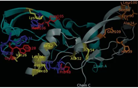
The second example is the bone morphogenetic pro-tein-2 (BMP-2), a member of the transforming growth fac-tor-b (TGF-b) with a pivotal role in bone formation and regeneration in adult vertebrates (Reddi, 1998). It signals by binding two types of serine/threonine kinase receptors, classified as type I and type II. Kirschet al.(2000) analyzed interactions of BMP-2 mutants with type I and type II re-ceptor ectodomains and found two different epitopes, each corresponding to a specific type of receptor. One epitope,

the strongest one, comprises residues from both monomers (Val:26, Asp:30, Trp:31, Lys:101, Tyr:103 from one mo-nomer and Ile:62, Leu:66, Asn:68, Ser:69, Phe:49, Pro:50, Ala:52 and His:54 from the other) while the other includes residues from only one monomer (Ala:34, His:39, Ser:88, Leu:90 and Leu:100).

In this example, we suppose that the epitopes in BMP-2 are unknown and we used our method for evaluat-ing all surface residues of a monomer. The analysis resulted in 29 residues predicted as hot spots, from a total of 101 sur-face residues. After that, we filtered the set of predicted res-idues using a sequential window of five adjacent resres-idues so that a positive prediction was kept only if among its two left and two right sequential neighbors at least two of them were also positive predictions. This kind of post-processing is quite common for interface region prediction methods (Yuanet al., 2004; Reset al., 2005). A total of 13 positive predictions survived this filtering process, 5 of them corre-sponding to residues in the first epitope (true positives). There were also 14 false negatives, 5 false positives and 83 true negatives, resulting in an F-Measure of 34.5% corre-sponding to a Precision of 50% and a Recall of 26.3%. If only the strongest epitope is considered, it results in an F-Measure of 43.5%, corresponding to a Precision of 50% and a Recall of 38.5%. Even though these levels of cover-age (Recall) are quite low, they are typical for interface re-gion prediction methods (Bradfordet al., 2006; Neuvirthet al., 2004) and, at a level of Precision of 50%, are considered as satisfactory for locating interface regions (Bradford and Westhead, 2005). Figure 3 summarizes these predictions. While no residue in the second epitope was found, all false positive predictions are close to those in the true positive in the first epitope.

Figure 2- One monomer from the tetramerization domain of the p53 tu-mor repressor (3sak:A). True positives are indicated in green, false posi-tives in purple and false negaposi-tives in yellow.

Concluding Remarks

In this work, we presented a method for predicting hot spot residues within the interface region. By using ROC analysis, we allow the user to choose the most appropriate trade off between true positive and false positive rates, ac-cording to his/her specific application. In addition, since the method does not depend on the knowledge of the struc-ture of the protein in complex, it can also be used in situa-tions where the interface region is unknown. Despite these advantages, the performance achieved by the method was also higher than those reported by previous studies using the same dataset.

References

Ahmed S, Gromiha M, Fawareh H and Sarai A (2004) ASAView: Database and tool for solvent accessibility representation in proteins. BMC Bioinform 5:51.

Altschul SF, Madden TL, Schäffer AA, Zhang J, Zhang Z, Miller W and Lipman DJ (1997) BLAST and PSI-BLAST: A new generation of protein database search programs. Nucleic Acids Res 25:3389-3402.

Apweiler R, Bairoch A, Wu CH, Barker WC, Boeckmann B, Ferro S, Gasteiger E, Huang H, Lopez R, Magrane M,et al. (2004) UniProt: The universal protein knowledgebase. Nu-cleic Acids Res 32:D115-D119.

Arkin MR and Wells JA (2004) Small-molecule inhibitors of pro-tein-protein interactions: Progressing towards the dream. Nat Rev Drug Discov 3:301-317.

Ban YA, Edelsbrunner H and Rudolph J (2006) Interface surfaces for protein-protein complexes. J ACM 53:361-378. Bogan AA and Thorn KS (1998) Anatomy of hot spots in protein

interfaces. J Mol Biol 280:1-9.

Bradford JR and Westhead DR (2005) Improved prediction of protein-protein binding sites using a support vector ma-chines approach. Bioinformatics 21:1487-1494.

Bradford JR, Needham CJ, Bulpitt AJ and Westhead DR (2006) Insights into protein-protein interfaces using a Bayesian net-work prediction method. J Mol Biol 362:365-386.

Cristianini N and Shawe-Taylor J (2000) An Introduction to Sup-port Vector Machines and other Kernel-based Learning Me-thods. 1st ddition. Cambridge University Press, Cambridge, 189 pp.

Darnell SJ, Page D and Mitchell JC (2007) An automated deci-sion-tree approach to predicting protein interaction hot spots. Proteins 68:813-823.

DeLano WL (2002) Unraveling hot spots in binding interfaces: Progress and challenges. Curr Opin Struct Biol 12:14-20. Duda RO, Hart PE and Stork DG (2001) Pattern Classification.

2nd edition. John Wiley & Sons, New York, 654 pp. Eisenberg D and McLachlan AD (1986) Solvation energy in

pro-tein folding and binding. Nature 319:199-203.

el-Deiry WS, Kern SE, Pietenpol JA, Kinzler KW and Vogelstein B (1992) Definition of a consensus binding site for p53. Nat Genet 1:45-49.

Fawcett T (2006) An introduction to ROC analysis. Pattern Recogn Lett 27:861-874.

Fernández-Recio J, Totrov M and Abagyan R (2004) Identifica-tion of protein-protein interacIdentifica-tion sites from docking energy landscapes. J Mol Biol 335:843-865.

Frishman D and Argos P (1995) Knowledge-based protein sec-ondary structure assignment. Proteins 23:566-579. Guney E, Tuncbag N, Keskin O and Gursoy A (2008) HotSprint:

Database of computational hot spots in protein interfaces. Nucleic Acids Res 36(Database issue):D662-D666. Hagerty CG, Munchnik I and Kulikowski C (1999) Two indices

can approximate four hundred and two amino acid proper-ties. Proc IEEE Int Simp Intell Cont, Intell Syst and Semio-tics, Cambridge, pp 365-369.

Hamelryck T and Manderick B (2003) PDB file parser and struc-ture implemented in python. Bioinformatics 19:2308-2310. Hanley JA and McNeil BJ (1982) The meaning and use of the area under a roc operating characteristic (ROC) curve. Radiology 143:29-36.

Hastie T and Tibshirani R (1998) Classification by pairwise cou-pling. In: Jordan MI, Kearns MJ and Solla SA (eds) Ad-vances in Neural Information Processing Systems 10. MIT Press, Cambridge, pp 507-513.

Higa RH and Tozzi CL (2008) Prediction of protein-protein bind-ing hot spots: A combination of classifiers approach. In: Bazzan ALC, Craven M and Martins NF (eds) Advances in Bioinformatics and Computational Biology. Third Brazilian Symposium on Bioinformatics, BSB 2008. Proceedings, LNCS 5167, pp 165-168.

Higgins D, Thompson J, Gibson T, Thompson JD, Higgins DG and Gibson TJ (1994). CLUSTAL W: Improving the sensi-tivity of progressive multiple sequence alignment through sequence weighting, position-specific gap penalties and weight matrix choice. Nucleic Acids Res 22:4673-4680. Hu Z, Ma B, Wolfson H and Nussinov R (2000) Conservation of

polar residues as hot spots at protein interfaces. Proteins 39:331-342.

Jones S and Thornton JM (1997) Analysis of protein-protein inter-action sites using surface patches. J Mol Biol 272:121-132. Kato S, Yin SY, Liu W, Otsuka K, Shibata H, Kanamaru R and

Ishioka C (2003) Understanding the function-structure and function-mutation relationships of p53 tumor suppressor protein by high-resolution missense mutation analysis. Proc Natl Acad Sci USA 100:8424-8429.

Kidera A, Konishi Y, Ooi T and Scheraga HA (1985) Relation be-tween sequence similarity and structural similarity in pro-teins. Role of important properties of amino acids. J Protein Chem 4:265-297.

Kirsch T, Nickel J and Sebald W (2000) BMP-2 antagonists emerge from alterations in the low-affinity binding epitope for receptor BMPR-II. EMBO J 19:3314-3324.

Koenderink JJ (1990) Solid Shape. MIT Press, Cambridge, 715 pp.

Kortemme T and Baker D (2002) A simple physical model for binding energy hot spots in protein-protein complexes. Proc Natl Acad Sci USA 99:14116-14121.

Li X, Keskin O, Ma B, Nussinov R and Liang J (2004) Pro-tein-protein interactions: Hot spots and structurally con-served residues often locate in complemented pockets that pre-organized in the unbound states. J Mol Biol 344:781-795.

Ma B, Elkayam T, Wolfson H and Nussinov R (2003) Pro-tein-protein interactions: Structurally conserved residues distinguish between binding sites and exposed protein sur-faces. Proc Natl Acad Sci USA 100:5772-5777.

McIvor AM and Valkenburg RJ (1997) A comparison of local sur-face geometry estimation methods. Mach Vision Appl 10:17-26.

Moreira IS, Fernandes PA and Ramos MJ (2007) Hot Spots - A re-view of the protein-protein interface determinant amino-acid residues. Proteins 68:803-812.

Neuvirth H, Raz R and Schreiber G (2004) ProMate: A structure based prediction program to identify the location of pro-tein-protein binding sites. J Mol Biol 338:181-199. Platt J (2000) Probabilistic outputs for support vector machines

and comparison to regularized likelihoods methods. In: Smola A, Bartlett P, Schölkpf B and Schuurmans D (eds) Advances in Large Margin Classifiers. MIT Press, Cam-bridge, pp 61-74.

Pupko R, Bell RE, Mayrose I, Glaser F and Ben-Tal N (2002) Rate4Site: An algorithmic tool for the identification of func-tional regions in proteins by surface mapping of evolution-ary determinants within their homologues. Bioinformatics 18:S71-S77.

Reddi AH (1998) Role of morphogenetic proteins in skeletal tis-sue engineering and regeneration. Nat Biotechnol 16:247-252.

Res I, Mihalek I and Lichtarge O (2005) An evolution based clas-sifier for prediction of protein interfaces without using pro-tein structures. Bioinformatics 21:2496-2501.

Rost B (1999) Twilight zone of protein sequence alignments. Pro-tein Eng 12:85-94.

Wesson L and Eisenberg D (1992) Atomic solvation parameters applied to molecular dynamics of proteins in solution. Pro-tein Sci 1:227-235.

Yuan C, Dobbs D and Honavar V (2004) A two-stage classifier for identification of protein-protein interface residues. Bioinformatics 20:i371-i378.

Internet Resource

Chang CC and Lin CJ (2001) LibSVM: A Library for Support

Vector Machines,

http://www.csie.ntu.edu.tw/~cjlin/libsvm. (June 10, 2008).

Guest Editor: José Carlos Merino Mombach