ISSN 0104-6632 Printed in Brazil
Vol. 19, No. 03, pp. 319 - 334, July - September 2002
Brazilian Journal
of Chemical
Engineering
MODELING AND SIMULATION OF A
PSEUDO-TWO-PHASE GAS-LIQUID COLUMN REACTOR
FOR THERMAL HYDROCRACKING OF
PETROLEUM HEAVY FRACTIONS
E.M.Matos and R.Guirardello
Universidade Estadual de Campinas , UNICAMP, Faculdade de Engenharia Química, Departamento de Processos Químicos, Cx.P. 6066, CEP 13081-970, Phone +55 (19) 3788-3955, Fax: +55 (19) 3788-3965, Campinas - SP, Brazil
E-mail: [email protected], E-mail: [email protected]
(Received: December 03, 2001 ; Accepted: June 11, 2002)
Abstract - This work presents a model to predict the behavior of velocity, gas holdup and local concentration fields in a pseudo-two-phase gas-liquid column reactor applied for thermal hydrocracking of petroleum heavy fractions. The model is based on the momentum and mass balances for the system, using an Eulerian-Eulerian approach. Using the k-ε model, fluid dynamics accounts for both laminar and turbulent flows, with discrete small bubbles (hydrogen) flowing in a continuous pseudohomogeneous liquid phase (oil and catalyst particles). The petroleum is assumed to be a mixture of pseudocomponents, grouped by similar chemical structural properties, and the thermal hydrocracking is taken into account using a kinetic network based on these pseudocomponents.
Keywords: slurry bubble column, reactor, hydrocracking, heavy oil, modeling.
INTRODUCTION
Three-phase and two-phase flow column reactors have many applications in industry. One of them is in the hydrocracking process, where large molecules of petroleum in the presence of excess hydrogen are broken into smaller molecules. In this process there is an increase in the amount of valuable oil subproducts, which is of great economic importance. The modeling and simulation of such reactors are quite complex, since they need to take into account both the fluid dynamics and the reactions that occur. There are a number of works in the literature about the modeling of these reactors (Celik and Wang, 1994; Chen et al, 1995; Gasche et al, 1990; Grienberger and Hofmann, 1992; Hillmer et al,
1994; Torvik and Svendsen, 1990), but they are usually applied to a different set of reactions. The present work presents a model that considers these features, specifically applied to the hydrocracking of oils, using some reasonable approximations in order to solve the problem numerically. The oil, which is a complex mixture of many compounds, is assumed to be a mixture of a small number of pseudocomponents, so that the reaction network is based on these pseudocomponents.
(liquid phase) and the catalyst particles (solid phase).
The hydrocracking modeled in this work is assumed to be thermal. The catalyst is only used to promote other kind of reactions, such as the removal of heteroatoms. However, the presence of the catalyst does affect the fluid dynamics. Considering that the catalyst particles are very small and have a small terminal velocity, in this work the slurry (oil + solid catalyst) was assumed to be a pseudo-homogeneous liquid phase.
MATHEMATICAL MODEL
The Kinetic Network
The hydrocracking reactions considered here are
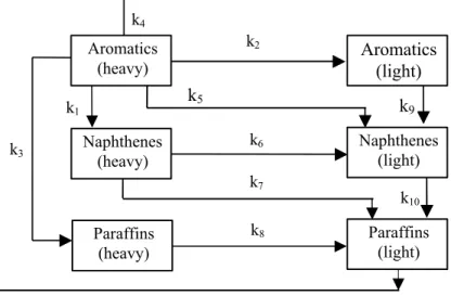
based on the kinetic network proposed by Krishna and Saxena (1989), established in terms of pseudocomponents, as shown in Figure 1. A pseudocomponent contains a set of molecules that have similar chemical structures. The aromatic lump is the pseudocomponent formed by the set of all molecules that have at least one benzenic ring in their structure. The naphthene lump is the pseudocomponent formed by the set of all molecules that have at least one cyclic ring in their structure that is not a benzenic ring. The paraffin lump is the pseudocomponent formed by the set of all molecules that do not have rings in their structure. The pseudocomponents are considered light if they are formed by fractions with boiling points not greater than some cut temperature; otherwise they are considered heavy. The values for the constants of reaction are given by Krishna and Saxena (1989).
Figure 1: The kinetic network
Assumptions
In this study, the following assumptions were made:
i) steady state process;
ii) uniform cross section for the reactor (cylinder); iii) uniform temperature inside the reactor
(isothermal);
iv) pseudo-two-phase model (slurry + gas); v) uniform density for the liquid phase;
vi) excess hydrogen in the gas phase and oil completely saturated with dissolved hydrogen (so that rates of reactions do not explicitly depend on the partial pressure of hydrogen).
Since the catalyst particles considered in this work are very small, the solid and liquid phases were assumed to be a pseudohomogeneous slurry phase. However, the solid phase does not enter or leave the reactor, since it remains confined within it. In this work we have not calculated the solid distribution inside the reactor. We have only considered that the solid concentration in the slurry is uniform, which means
s s s l
f +
ε =
ε ε ∀ r, z (1)
where f is the average solid concentration in the s
slurry inside the reactor. Naphthenes
(light) k3
k1
Aromatics (heavy)
k9
k10
Aromatics (light)
Naphthenes (heavy)
Paraffins (heavy)
Paraffins (light) k2
k5
k6
k7
k8
The density and the holdup of the slurry phase are given by
s s l l sl
s l
ε ⋅ρ + ε ⋅ρ ρ =
ε + ε (2)
sl s l
ε = ε + ε (3)
For laminar flows, the viscosity for the slurry phase is given by (Hillmer et al., 1994)
(
)
(
)
(
)
2.59sl l 1 s s l s 1 s −
µ = µ ⋅ + ε ρ − ρ ρ ⋅ − ε (4)
For turbulent flows, the k-ε model was used to
calculate the turbulent viscosity. The effective viscosity is given by
eff ,k k t,k
µ = µ + µ k=g,sl (5)
t,k t,k
k
µ
ν =
ρ k=g,sl (6)
(
)
2
t,g t,sl Rp 1 5 s
ν = ν ⋅ ⋅ + ε (7)
In this work, the value of R was assumed to be 1. p
The dispersion coefficient can be calculated by (Hillmer et al., 1994)
r,k t,k
D = ν k=g,sl (8)
z,k t,k
D = ν k=g,sl (9)
Mass Balance Equations
Since we are modeling the oil fractions as pseudocomponents, all concentrations and rates of reaction will be expressed on a mass basis. Therefore, the mass rates per unit volume of liquid
(not slurry) r satisfy the equation i
Nc i i 1
r 0
=
=
∑
(10)where ri>0 for formation and ri <0 for
consumption.
Gas Phase (Mainly Hydrogen)
(
) (
)
2
g g
r,g g z,g g
g g r,g g g z,g
H v P v
1
r D D
r r r z z
1
r v v
r r z
N a N a
∂ ε ∂ ε
∂ ∂
− ⋅∂ ⋅ ⋅ρ ⋅ ∂ −∂ ⋅ρ ⋅ ∂ +
∂ ∂
⋅ ⋅ρ ⋅ε ⋅ + ρ ⋅ε ⋅ =
∂ ∂ − ⋅ + ⋅ (11) where 2 H
N and N are the mass transfer rates of P
hydrogen and products between gas and slurry phases, respectively. Since in this model we are assuming a large excess of hydrogen, these two terms were neglected.
The dispersion of the gas phase (small bubbles) is caused mainly by the turbulence in the slurry phase. For laminar flows, the dispersion terms are zero. For turbulent flows, all variables and properties are time averaged.
Slurry Phase
Under the previously mentioned assumptions, the global mass balance for the slurry phase results in the following equation:
(
)
(
)
2sl r,sl sl
sl
z,sl sl sl sl r,sl
sl sl z,sl H v P v
1
r D
r r r
1
D r v
z z r r
v N a N a
z
∂ ε
∂
− ⋅ ⋅ ⋅ρ ⋅ −
∂ ∂
∂ ε
∂ ∂
− ⋅ρ ⋅ + ⋅ ⋅ρ ⋅ε ⋅ +
∂ ∂ ∂
∂
+ ρ ⋅ε ⋅ = ⋅ − ⋅
∂
(12)
where
2
H
N and N are the mass transfer rates of P
hydrogen and products between gas and slurry phases, respectively. These two terms were also neglected in this equation, because they are smaller than the others.
The mass balance for each pseudocomponent j in the slurry phase, based on the kinetic network in Figure 1, is given by
(
)
(
)
(
)
(
)
r,sl sl j,sl sl
z,sl sl j,sl sl
j,sl sl r,sl
j,sl sl z,sl j,sl sl j v
1
r D
r r r
D
z z
1
r v
r r
v r N a
z
∂ ∂
− ⋅ ⋅ ⋅ρ ⋅ ω ⋅ ε −
∂ ∂
∂ ∂
− ⋅ρ ⋅ ω ⋅ ε +
∂ ∂
∂
+ ⋅ ⋅ρ ⋅ε ⋅ +
∂ ∂
+ ρ ⋅ ε ⋅ = ⋅ ε + ⋅
∂
where ωj,sl is the mass fraction of j in the slurry,
j,sl
r is the rate of reaction of j in the slurry and N j
is the mass transfer rate of each pseudocomponent j between gas and slurry phases. These mass transfer terms were also neglected in this equation.
It is important to note that the summation of equation (13) over all species in the slurry (dissolved hydrogen, solid catalyst, pseudocomponents) should result in equation (12), the global mass balance for the slurry phase.
It is desirable to express the concentration of j in mass of j/volume of liquid phase and not slurry, since the rates of reaction are usually expressed in the liquid phase. It can easily be shown that
j,sl sl j l
ρ ⋅ε = ρ ⋅ ε (14)
j,sl sl j l
r ⋅ ε = ⋅ εr (15)
and since ρsl and f (equation 1) are considered s
constants in this model, equation (13) can be written as
(
)
(
)
(
)
(
)
r,sl j l
z,sl j l
j l r,sl
j l z,sl j l j v
1
r D
r r r
D
z z
1
r v
r r
v r N a
z
∂ ∂
− ⋅ ⋅ ⋅ ρ ⋅ε −
∂ ∂
∂ ∂
− ⋅ ρ ⋅ε +
∂ ∂
∂
+ ⋅ ⋅ρ ⋅ ε ⋅ +
∂
∂
+ ρ ⋅ ε ⋅ = ⋅ ε + ⋅
∂
(16)
Using the kinetic network shown in Figure 1, the reaction rates for the pseudocomponents are given by
Heavy Aromatics
Ah 1 2 3 4 5 Ah
r = −(k +k +k +k +k )⋅ρ (17)
Light Aromatics
Al 2 Ah 9 Al
r =k ⋅ρ −k ⋅ρ (18)
Heavy Naphthenes
Nh 1 Ah 6 7 Nh
r = ⋅ρk −(k +k )⋅ρ (19)
Light Naphthenes
Nl 5 Ah 9 Al 6 Nh 10 Nl
r =k ⋅ρ +k ⋅ρ +k ⋅ρ −k ⋅ρ (20)
Heavy Paraffins
Ph 3 Ah 8 Ph
r =k ⋅ρ −k ⋅ρ (21)
Light Paraffins
Pl 4 Ah 7 Nh 10 Nl 8 Ph
r =k ⋅ρ +k ⋅ρ +k ⋅ρ +k ⋅ρ (22)
An equation similar to (13) may be written for the hydrogen in the liquid phase. Since excess hydrogen is present in the gas phase at a high pressure, flowing as small bubbles, it was assumed that mass transfer coefficients between phases were high enough so that
2
H
ρ in the liquid phase was
close to the equilibrium concentration and uniformly distributed. Therefore, the mass balance for hydrogen in the liquid may be written as
2 2
l rH NH av 0
ε ⋅ + ⋅ = (23)
If we try to calculate the rate of consumption of hydrogen in the liquid phase, using equation (10), we get the following unrealistic result:
2
H Ah Al Nh Nl Ph Pl
r = −(r +r +r +r +r +r )=0 (24)
because we are assuming that 1 kg of component p converts into 1 kg of component q. Unless we have information about the average molecular weight of each pseudocomponent and the average stoichiometric ratio between pseudocomponents, this model does not allow calculation of the rate of consumption of hydrogen.
Momentum Balance Equations
The momentum and force balances for the system, under the previously mentioned considerations, are given by the following equations (Torvik and Svendsen, 1990), considering gravitational forces in the z direction only.
Gas Phase
(
)
(
)
(
)
(
)
(
)
g g r,g z,g g g z,g z,g g
g zr,g g zz,g g g I,z z
1
r v v v v P
r r z z
1
r g F M
r r z
∂ ∂ ∂
⋅ ⋅ρ ⋅ε ⋅ ⋅ + ρ ⋅ ε ⋅ ⋅ = − ε ⋅ −
∂ ∂ ∂
∂ ∂
− ⋅ ⋅ε ⋅ τ − ε ⋅ τ − ε ⋅ρ ⋅ − −
∂ ∂
(25)
Radial Component
(
)
(
)
(
)
(
)
(
) (
)
g g r,g r,g g g z,g r,g g
g rr,g g rz,g g ,g I,r M r
1
r v v v v P
r r z r
1 1
r F F M
r r z r θθ
∂ ∂ ∂
⋅ ⋅ρ ⋅ε ⋅ ⋅ + ρ ⋅ ε ⋅ ⋅ = − ε ⋅ −
∂ ∂ ∂
∂ ∂
− ⋅ ⋅ε ⋅ τ − ε ⋅ τ + ⋅ ε ⋅ τ − − −
∂ ∂ (26) Slurry Phase Axial Component
(
)
(
)
(
)
(
)
(
)
sl sl r,sl z,sl sl sl z,sl z,sl
sl sl zr,sl sl zz,sl sl sl I,z z
1
r v v v v
r r z
1
P r g F M
z r r z
∂ ∂
⋅ ⋅ρ ⋅ε ⋅ ⋅ + ρ ⋅ ε ⋅ ⋅ =
∂ ∂
∂ ∂ ∂
= − ε ⋅ − ⋅ ⋅ ε ⋅ τ − ε ⋅ τ − ε ⋅ρ ⋅ + +
∂ ∂ ∂
(27)
Radial Component
(
)
(
)
(
)
(
)
(
) (
)
sl sl r,sl r,sl sl sl z,sl r,sl sl
sl rr,sl sl rz,sl sl ,sl I,r M r
1
r v v v v P
r r z r
1 1
r F F M
r r z r θθ
∂ ∂ ∂
⋅ ⋅ρ ⋅ε ⋅ ⋅ + ρ ⋅ε ⋅ ⋅ = − ε ⋅ −
∂ ∂ ∂
∂ ∂
− ⋅ ⋅ε ⋅ τ − ε ⋅ τ + ⋅ ε ⋅ τ + + +
∂ ∂
(28)
where
(
)
I,z W g sl z,g z,sl
F =C ⋅ ε ⋅ε ⋅ v −v (29)
(
)
I,r W g sl r,g r,sl
F =C ⋅ ε ⋅ ε ⋅ v −v (30)
(
)
z,slM M g sl sl z,g z,sl
v
F C v v
r
∂
= − ⋅ε ⋅ε ⋅ρ ⋅ − ⋅
∂ (31)
(
2)
z v H z,g P z,sl
M =a ⋅ N ⋅v −N ⋅v (32)
(
2)
r v H r,g P r,sl
M =a ⋅ N ⋅v −N ⋅v (33)
r,k rr,k eff ,k
v 2
r
∂
τ = −µ ⋅ ⋅
∂
(34)
z,k zz,k eff ,k
v 2
z
∂
τ = −µ ⋅ ⋅
∂
(35)
,k eff ,k r,k
1
2 v
r
θθ
τ = −µ ⋅ ⋅ ⋅
(36)
z,k r,k rz,k zr,k eff ,k
v v
r z
∂ ∂
τ = τ = −µ ⋅ +
∂ ∂
(37)
where
k=g,sl.
Turbulent Flow
For turbulent flow, the k-ε model was used to
(
sl sl r,sl sl)
(
sl sl z,sl sl)
sl sl
eff ,sl sl eff ,sl sl k,sl sl
1
r v k v k
r r z
k k
1
r S
r r r z z
∂ ∂
⋅ ⋅ρ ⋅ ε ⋅ ⋅ + ⋅ ρ ⋅ ε ⋅ ⋅ =
∂ ∂
∂ ∂
∂ ∂
= ⋅ ⋅µ ⋅ ε ⋅ + µ ⋅ ε ⋅ + ⋅ε
∂ ∂ ∂ ∂
(38)
where
(
)
k,sl sl sl d,sl
S = G − ρ ⋅ ε (39)
(
sl sl r,sl d,sl)
(
sl sl z,sl d,sl)
eff ,sl d,sl eff ,sl d,sl
sl sl e,sl sl
1
r v v
r r z
1
r S
r r 1.3 r z 1.3 z
∂ ∂
⋅ ⋅ρ ⋅ ε ⋅ ⋅ ε + ⋅ ρ ⋅ ε ⋅ ⋅ ε =
∂ ∂
µ ∂ ε µ ∂ ε
∂ ∂
= ⋅ ⋅ ⋅ε ⋅ + ⋅ε ⋅ + ⋅ ε
∂ ∂ ∂ ∂
(40)
where
(
)
d,sl
e,sl sl sl d,sl
sl
S 1.44 G 1.92
k
ε
= ⋅ ⋅ − ⋅ρ ⋅ε
(41)
and
2 2 2 2
z,sl r,sl r,sl r,sl z,sl
sl t,sl
v v v v v
G 2
z r r z r
∂ ∂ ∂ ∂
= µ ⋅ ⋅ ∂ + ∂ + + ∂ + ∂
(42)
The turbulent viscosity for the slurry phase is calculated from
2 sl
t,sl sl
d,sl
k 0.09
µ = ⋅ρ ⋅
ε (43)
The turbulent viscosity for the gas phase is calculated from equations (6) and (7), using the turbulent viscosity for the slurry phase.
Boundary Conditions
For this work, the slurry is assumed to be leaving the reactor uniformly at the lateral position at the top
of the reactor ( r=R, z=L), while the gas is
assumed to be leaving the reactor at the top ( z=L,
0≤ ≤r R). This is in fact an approximation, and the
actual area for the slurry outlet is given by a small area at the lateral position. At the inlet, both slurry
and gas phases enter at the bottom ( z=0,
0≤ ≤r R).
The boundary conditions for equations (11) – (12) and (25) – (28) are given by
e z,k z,k
v =v z=0 0≤ ≤r R (44)
r,k
v =0 z=0 0≤ ≤r R (45)
z,sl
v =0 z=L 0≤ ≤r R (46)
z,g
v 0 z
∂ =
∂ z=L 0≤ ≤r R (47)
r,sl
v 0 z
∂ =
∂ z=L 0≤ <r R (48)
r,g
v 0 z
∂ =
∂ z=L 0≤ ≤r R (49)
z,k
v 0 r
∂ =
r,k
v =0 r=0 0≤ ≤z L (51)
z,k
v =0 r=R 0≤ ≤z L (52)
r,sl
v =0 r=R 0≤ <z L (53)
r,g
v =0 r=R 0≤ ≤z L (54)
where k=g,sl. Observe that the limits for the
intervals for conditions (48) and (53) do not apply
for vr,sl at z=L and r=R.
The boundary conditions for equation (16) are given by
j
0 r
∂ ρ =
∂ r=0 0≤ ≤z L (55)
j
0 r
∂ ρ =
∂ r=R 0≤ ≤z L (56)
e j j
ρ = ρ z=0 0≤ ≤r R (57)
j
0 z
∂ ρ =
∂ z=L 0≤ ≤r R (58)
For laminar flows conditions (44) and (45) in the wall work fine. However, for turbulent flows the velocity gradients near the wall are very high, making it very difficult to calculate numerically the velocity profiles. So, instead of condition (44), for turbulent flows the Prandtl logarithmic law is used as a boundary condition near the wall (Launder and Spalding, 1974):
w,k k w,k k
z,k
k k
v ln E y
0.42
τ ρ τ ρ
= ⋅ ⋅ ⋅
µ ρ
(59)
where y= −R r is the distance from the wall and
w,k
τ is the wall stress (equation (38) for r=R),
which can be related to the pressure gradient by integrating equations (25) and (27).
For the k-ε model, the boundary conditions near
the wall are (Xu et al., 1998)
(
)
2w,sl sl sl
k
0.09
τ ρ
= (60)
(
)
3w,sl sl d,sl
0.42 y
τ ρ
ε =
⋅ (61)
Model Resolution
The equations were discretized by applying the finite volume method, which converted the nonlinear equations into a linearized system that was solved by LU decomposition (in each iteration). The staggered grid scheme was used to locate the variables in the control volumes. The upwind scheme for convective terms and the central difference for diffusive terms were used to avoid negative coefficients and a consequently numerical instability. The source terms were linearized in such a way as to ensure that the matrix coefficients were diagonally dominant.
Due to strong nonlinearities, the velocity (momentum) and holdup equations must be underrelaxed and a specific sequence in solving the equations must be obeyed to get convergence (Patankar, 1980).
The gas holdup was evaluated by combination of the continuity equations for the two phases, subtracting one from the other. For the pressure correction, the SIMPLEC method was used (Maliska, 1995), adding up the continuity equations for the two phases.
The model was solved in 12 x 12 grid, using C as the programming language. The criteria for convergence used in the iterative procedure was:
13 13
(n 1) (n) 9
ij ij
i 2 j 2
P + P 10−
= =
− ≤
∑ ∑
(62)Except pressure, all variables are specified at the inlet of the reactor. All velocities are zero at the wall, since it is impermeable for gas and slurry. At the centerline, radial velocities and the deviates of all variables are zero. At the free surface (end of the reactor), all gradients were set to zero. The outlet velocities are calculated in such a way that the mass balance must be obeyed.
an arbitrary reference value of pressure equal to zero was set at the last numbered point in the grid.
About the pressure term in the momentum
equations, either form
(
ε ⋅∇k P)
or ∇ ε ⋅(
k P)
may beused in equations because both satisfy the condition that, when the corresponding momentum equations for the two phases are added, the resulting pressure
gradient must be P∇ (Celik and Wang, 1994).
The value for CW in equations (29) and (30) was
given by (Grienberger and Hofmann, 1992):
(
)
W
C =50000 2.2 1.7⋅ − ⋅ r R (63)
in kg/m3.s, considering a variation with radial
position in order to get a better agreement between experimental and calculated values.
Some approximations were also used to solve the model. The mass transfer between gas and liquid phases was neglected, considering that the hydrogen was present in excess and assuming that the more volatile hydrocarbons remained dissolved in the oil, due to the high pressure. The oil density was assumed to be constant inside the reactor, thus neglecting some of the effects of reaction in the fluid dynamics. Also, the hydrogen density was assumed to be constant, since the pressure drop was much smaller than the absolute pressure in the reactor (around 100 atm).
NUMERICAL RESULTS
Air-Water System
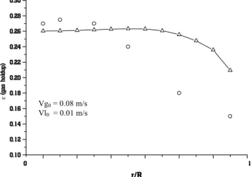
In order to test the performance of the model, numerical results were compared with experimental data available from the literature. Figure 2 shows
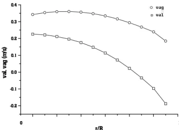
experimental results from an air-water system (Grienberger & Hofmann, 1992) comparing the gas holdup profile in the radial direction with numerical results for the same operating conditions. Figure 3 shows experimental results from an air-water system (Gasche et al., 1990), comparing the gas velocity profile in the radial direction with numerical results for the same operating conditions. Figure 4 shows experimental results from an air-water system (Torvik and Svendsen, 1990), comparing the liquid velocity profile in the radial direction with numerical results for the same operating conditions. In all figures, the squares represent calculated values, while circles represent experimental values. The indicated inlet velocities are the superficial velocities, given by the mass flow of each phase divided by the phase density and the area of cross section of the reactor. In order to get the actual inlet velocities, these values must be divided by the inlet holdup of each phase. In all figures, the profiles were calculated for h = 2.25 m, the middle height of the column, in order to avoid inlet and outlet effects.
It can be observed from the figures that in some cases the numerical results are close to the experimental data (Figures 2 and 3), while in others they are not (Figure 4). However, in all cases the physical behavior is qualitatively correct.
The fluid-dynamic variables (liquid and gas velocities, gas and liquid holdups) influence the mass balance by affecting the residence time and the mixing of the components. When the internal velocities are very high, the physical behavior of the reactor approaches the perfect mixing reactor (CSTR). However, the recirculating movement of the slurry phase leads to dead zones, so that it is important to study the fluid-dynamic profiles in order to get a better understanding of reactor behavior.
2 4 6 8 10 12 14
0.10 0.12 0.14 0.16 0.18 0.20 0.22 0.24 0.26 0.28 0.30
ε
(
ga
s
ho
ld
up
)
0 1
r/R
Figure 2: Variation in gas holdup with radial position Vg0 = 0.08 m/s
2 4 6 8 10 12 14
-0.1 0.0 0.1 0.2 0.3 0.4 0.5
0 1
v
ag
(
m
/s
)
r/R
Figure 3: Variation in gas axial velocity with radial position
2 4 6 8 10 12 14
-0.4 -0.2 0.0 0.2 0.4 0.6
0 1
V
al
(
m
/s
)
r/R
Figure 4: Variation in liquid axial velocity with radial position
Hydrogen-Oil System
The values for the parameters used in the model are shown in Table 1. The kinetic constants were taken from Krishna and Saxena (1989) for a cut
temperature of 700 °F (to distinguish heavy from
light). As in Hillmer et al. (1994), the dispersion coefficients were expressed in terms of viscosity.
The value for CM was taken from Torvik and
Svendsen (1990), while the value for C was W
calculated by equation (63). The other parameter values were arbitrarily set.
In the numerical simulations, the inlet liquid phase superficial velocity was set to 0.01 m/s, while gas phase superficial velocity at the reactor inlet was 0.08 m/s. The inlet gas holdup was 0.25, while inlet oil holdup was 0.75. The solid catalyst was assumed to be confined inside the reactor. The reactor inner
diameter was 0.3 m and the total length of the reactor was 4.5 m.
The oil density was assumed to be 660 kg/m3,
while the catalyst density was assumed to be 1660
kg/m3, both at the operating conditions. The slurry
density depends on the value of f (equations (1) s
and (2)), so that for f equal to 0.14 the slurry s
density is 800 kg/m3 and for f equal to 0.34 the s
slurry density is 1000 kg/m3.
The numerical results are shown in Figures 5 through 14. In all figures the slurry density was 800
kg/m3, with the exception of Figures 8 and 9, which
also used slurry density 1000 kg/m3. Whenever not
stated in the figures, for profiles with radial variation the fixed axial position is the middle of the column (h = 2.25 m) and for profiles with axial variation the fixed radial position is the center of the column (r = 0).
Vg0 = 0.04 m/s
Vl0 = 0.00 m/s
Vg0 = 0.08 m/s
Figure 5 shows the variation in gas holdup with radial position for two different heights (axial position) inside the reactor. This figure shows that the gas is more concentrated in the center of the reactor, which is usually observed in this kind of reactor.
Figure 6 shows the variation of slurry axial velocity with radial position for two different heights (axial position) inside the reactor. This figure shows the upward movement in the center of the column and the downward movement close to the wall, which is also usually observed in this kind of reactor.
Figure 7 shows the variation in axial velocities with radial position for liquid and gas. This figure shows that gas velocity is higher than slurry velocity, due to the higher volumetric flow of hydrogen than oil.
Figure 8 shows the variation in gas holdup with radial position for two different slurry densities (800
and 1000 kg/m3). This figure shows that the gas
holdup profile has only a small variation with the slurry density.
Figure 9 shows the variation in axial velocity with radial position for slurry for two different slurry
densities (800 and 1000 kg/m3). This figure shows
that the slurry axial velocity profile has only a small
variation with the slurry density.
Both Figures 8 and 9 indicate that the slurry density have a small effect in the fluid dynamics of the column. However, one should not conclude from that that gradients in oil or slurry densities inside the reactor would not change the fluid dynamics, because in the simulated cases we have assumed an uniform slurry density through the reactor, although with different values in each simulation.
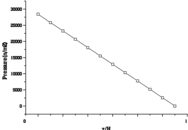
Figure 10 shows the variation in pressure with axial position (reactor height). This figure shows the expected drop in pressure with column height due mainly to the weight of the slurry.
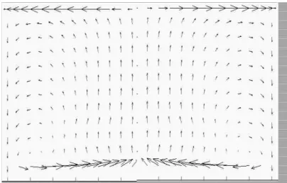
Figure 11 shows the fluid dynamic vector field for slurry, with the upward flow in the center of the reactor and downward flow close to the wall.
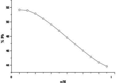
Figures 12 through 17 show the variation in concentration for each one of the pseudocomponents with axial position. As expected, the only pseudocomponent that increases its concentration is the light paraffin, because it is only produced in the kinetic network. The light naphtenics and light aromatics have a peak in concentration at the bottom of the reactor. All other pseudocomponents have a decrease in concentration.
Table 1: Parameter values used in the model simulation
Variable Units Value
k1 1/h 1.2633
k2 1/h 0.6042
k3 1/h 0.0421
k4 1/h 0.5309
k5 1/h 0.0397
k6 1/h 1.1855
k7 1/h 0.1619
k8 1/h 0.4070
k9 1/h 0.2909
k10 1/h 0.0818
0 Ah
ω % 2.0
0 Al
ω % 1.5
0 Nh
ω % 15.0
0 Nl
ω % 10.0
0 Ph
ω % 50.0
0 Pl
ω % 21.5
M
C -0.5
Figure 5: Variation in gas holdup with radial position
2 4 6 8 10 12 14
-0.2 -0.1 0.0 0.1 0.2 0.3
h = 1 m h = 4 m
0 1
v
al
(
m
/s
)
r/R
Figure 6: Variation in axial velocity with radial position for liquid
2 4 6 8 10 12 14
-0.2 -0.1 0.0 0.1 0.2 0.3 0.4
cw = 50000(2.2-1.7sqrt(r/R))
0 1
v
al
, v
ag
(
m
/s
)
r/R
2 4 6 8 10 12 14
0.25 0.26 0.27 0.28 0.29 0.30 0.31 0.32
0 1
εg
r/R
Figure 8: Variation in gas holdup with radial position
2 4 6 8 10 12 14
-0.2 -0.1 0.0 0.1 0.2 0.3
0 1
V
al
(
m
/s
)
r/R
Figure 9: Variation in axial velocity with radial position for liquid
2 4 6 8 10 12 14
0 5000 10000 15000 20000 25000 30000
0 1
P
re
ss
u
re
(n
/m
2)
z/H
Figure 10: Variation of pressure with axial position
ο slurry density: 1000 kg/m3 slurry density: 800 kg/m3
Figure 11: Fluid dynamic velocity field for slurry (not on scale)
2 4 6 8 10 12 14
1.5 1.6 1.7 1.8 1.9 2.0
0 1
%
A
h
z/H
Figure 12: Concentration of heavy aromatics with axial position
2 4 6 8 10 12 14
1.35 1.40 1.45 1.50 1.55 1.60
0 1
%
A
l
z/H
2 4 6 8 10 12 14
12.5 13.0 13.5 14.0 14.5 15.0 15.5
0 1
%
N
h
z/H
Figure 14: Concentration of heavy naphtenics with axial position
2 4 6 8 10 12 14
9.8 10.0 10.2 10.4 10.6 10.8 11.0
0 1
%
N
l
z/H
Figure 15: Concentration of light naphtenics with axial position
2 4 6 8 10 12 14
44 46 48 50 52
0 1
%
P
h
z/H
2 4 6 8 10 12 14
18 20 22 24 26 28 30 32
0 1
%
P
l
z/H
Figure 17: Concentration of light paraffins with axial position
CONCLUSIONS
The results show that the proposed model can be used to describe the behavior of a slurry bubble column reactor, in this case applied to a process of thermal hydroconversion of heavy oils. The fluid dynamic fields were based on momentum transfer and mass balances and are used to calculate the concentrations of the chemical species involved. The kinetic model, based on a pseudocomponent approach, is general and can be applied to different oils and different operating conditions. However, the specific values used in the simulations only apply to the operating conditions used to obtain the data taken from the literature.
The model has some limitations that can be improved, such as the calculations of hydrogen consumption, mass transfer coefficients between phases and solid dispersion inside the reactor.
The kinetic network can be extended to any oils, although compositional details of the heavy oil to be processed must be known. This model can be helpful for future work in optimization and control of the petroleum hydrocracking process, which is always seeks to increase economically the marketable fraction of petroleum.
ACKNOWLEDGMENTS
The authors would like to thank FAPESP, Fundação de Amparo à Pesquisa do Estado de São Paulo, for the funding that supported this research.
NOMENCLATURE
h
A heavy aromatics
l
A light aromatics
v
a interfacial area, m2/m3
Ci concentration of lump i, mol/cm
3
ci 0
inlet concentration of lump i, mol/cm3
Cm constant of radial force
Cw constant of interfacial drag force, kg/m
3
.s
z,k
D dispersion coefficient for phase k in
direction z , m2/s
r,k
D dispersion coefficient for phase k in
direction r , m2/s
E roughness factor
g gravitational constant, m2/s
k turbulent kinetic energy, J/kg
i
k constant of reaction for path i , 1/h
Nh heavy naphthenes
Nl light naphthenes
Ph heavy paraffins
Pl light paraffins
i
r rate of reaction for specie i , kg/s
r radial position, m
uz,g gas velocity, z-component, m/s
ur,g gas velocity, r-component, m/s
uz,l slurry velocity, z-component, m/s
ur,l slurry velocity, r-component, m/s
z
axial position, mdis
ε turbulence dissipation rate, J/kg.s
g
ε gas holdup, m3/m3
l
ε liquid holdup, m3/m3
s
ε solid holdup, m3/m3
sl
ε slurry holdup, m3/m3
eff ,k
µ effective viscosity of phase k , kg/m.s
k
µ viscosity of phase k , kg/m.s
t,k
µ turbulent viscosity of phase k , kg/m.s
t,k
ν kinematic turbulent viscosity of phase k ,
m2/s
g
ρ gas density, kg/m3
l
ρ liquid density, kg/m3
s
ρ solid density, kg/m3
sl
ρ slurry density, kg/m3
REFERENCES
Celik, I. and Wang, Y.Z., Numerical Simulation of Circulation in Gas-Liquid Column Reactors: Isothermal, Bubbly, Laminar Flow. Int. J. Multiphase Flow, vol. 20, nº 6, pp. 1053-1070, 1994.
Chen, Z., Zheng, C., Feng, Y. and Hofmann, H., Modelling of Three-phase Fluidized Beds Based on Local Bubble Characteristics Measurements, Chemical Engineering Science, vol. 50, n° 2, pp. 231-236, 1995.
Gasche, H.-E., Edinger, C., Kömpel, H. and Hofmann, H., A Fluid-dynamically Based Model of Bubble
Column Reactors, Chemical Engineering & Technology, 13, pp. 341-349, 1990.
Grienberger, J. and Hofmann, H., Investigations and Modeling of Bubble Columns, Chemical Engineering Science, 47 (9-11), pp. 2215-2220, 1992.
Hillmer, G., Weismantel, L. and Hofmann, H., Investigations and Modelling of Slurry Bubble Columns. Chemical Engineering Science, vol. 49, n° 6, pp. 837-843, 1994.
Krishna, R. and Saxena, A. K., Use of an Axial-dispersion Model for Kinetic Description of Hydrocracking. Chemical Engineering Science, vol. 44, n° 3, pp. 703-712, 1989.
Launder, B.E. and Spalding D.B., The Numerical Computation of Turbulent Flows. Comput. Methods Appl. Mech. Eng., 3, 269-289, 1974. Maliska, C.R., Transferência de Calor e Mecânica
dos Fluidos Computacional. Livros Tecnicos e Científicos Editora, 1995.
Mosby, J.F., Buttke, R.D., Cox, J. and Nikolaides, C., Process Characterization of Expanded-bed Reactors in Series, Chemical Engineering Science, vol. 41, n° 4, pp. 989-995, 1986.
Patankar, S.V., Numerical Heat Transfer and Fluid Flow, Hemisphere Publishing Corporation, pp. 67, 1980. Torvik, R. and Svendsen, H.F., Modelling of Slurry
Reactors – A Fundamental Approach, Chemical Engineering Science, vol. 45, nº 8, pp. 2325-2332, 1990.