Pesqui. Oper. vol.32 número3

(1)

Printed version ISSN 0101-7438 / Online version ISSN 1678-5142 www.scielo.br/pope

EX-ANTE_{ECONOMIC ASSESSMENT IN INCREMENTAL R&D PROJECTS:}

TECHNICAL AND DEVELOPMENT TIME UNCERTAINTIES ADDRESSED BY THE REAL OPTIONS THEORY

Luis Alberto Melchiades Leite

∗

, Jos´e Paulo Teixeira

and Carlos Patr´ıcio Samanez

Received September 13, 2011 / Accepted July 20, 2012

ABSTRACT.This paper analyzes changes in the assessment of an incremental R&D project by an indus-trial firm with the progressive consideration of the endogenous treatment of its main sources of uncertainty: technical performance and development time. We found that the project, which was unfeasible under a deterministic assessment by Net Present Value (NPV) without flexibility, became feasible after the treat-ment of the technical uncertainty by a real options model (NPV with flexibility). Moreover, the project gained approximately 51 percent more value in flexibility when a treatment of the development time un-certainty was added to the model. In terms of additional flexibility per unit cost of the project, the gain is approximately 44 percent. This result demonstrates the importance of addressing the combination of these sources of uncertainty in R&D projects, especially those that are incremental, which is a difficult category to analyze in terms of quantitative benefits.

Keywords: decision under uncertainty, real options in R&D, economic evaluation of R&D projects.

1 INTRODUCTION

Since the 1980s, the applicability of methodologies that are already well established in corpo-rate practice to the assessment of investment projects, with high degrees of uncertainty, has been discussed, as reported by Faulkner (1996) and Neves (1992). Research and development (R&D) projects are the quintessential representatives of this category of investments, in which the risk of additional factors to the natural uncertainties of the market (for example, technical uncer-tainty) leads to assessments made in conventional methodological bases, imposing a penalty that frequently induces companies to underinvest in R&D.

Conventional financial methods, based on the Net Present Value (NPV) of a Discounted Cash Flow (DCF), do not properly consider the presence of an extended risk, insofar as the latter

*Corresponding author

(2)

is wrongly addressed through an excessive raise in the discount rate. That raise often reaches a much higher level than that required for development projects without extended risk, which is normally defined by the firm’s cost of capital (Samanez, 2007). The assumption of active management in the presence of flexibility, along the useful life of a project (in which a manager periodically reassesses the partially controllable endogenous uncertainties and performs optimal actions, thus maximizing value), is a fundamental methodological characteristic that requires the inclusion of different instruments in the proposal to properly assess that special category of projects.

The Real Options Theory, as originally proposed by Dixit & Pindyck (1994), provides solutions for this problem. Since this milestone, hundreds of new different models have been proposed, improving investment analysis in general, with appropriate considerations regarding managerial flexibility. Trigeorgis (1996), Amram & Kulatilaka (1999) and Copeland & Antikarov (2001) presented interesting case studies, contributing to the spread of a more practical view of the theory. Even classical problems, such as capacity expansion investments, can be better examined by Real Options Theory, as shown by Novaes & Souza (2005). More recently, Batista et al. (2011) adopted a Real Options approach to calculate an incremental payoff for energy projects in the carbon market. A broad discussion of updated Real Options tools and techniques, along with many case studies, can be found in Mun (2006).

Models based on Real Options Theory properly consider the value of managerial flexibility in the presence of technical uncertainty, as in the model developed by Santiago & Vakili (2005). The application of real options to the assessment of R&D projects is not new. There are other, more analytical approaches, such as those applied by Santos & Pamplona (2002) and Schwartz (2001). Paxon (20003) organizes a relevant collection of articles addressing the problem in the same way, aiming to treat a number of challenges involving the evaluation of R&D projects. However, technical uncertainty is understood to be somewhat idiosyncratic, thus requiring a more specific treatment, as suggested by Huchzermeier & Loch (2001). According to these authors, there are five significant sources of uncertainty that affect the value of R&D projects: the performance of technology or technological development, the development time, the level of demand from the market and how much it pays for each level of technological performance (market payoff). Silva & Santiago (2009) proposed an interesting alternative approach to the consideration of the development time, by considering it in a stochastic way in the decision-making model calcu-lated by dynamic programming, unlike the method used by Huchzermeier & Loch (2001) and Crespo (2008).

(3)

LUIS ALBERTO MELCHIADES LEITE, JOS ´E PAULO TEIXEIRA and CARLOS PATR´ICIO SAMANEZ

619

engineering knowledge basis, according to Rousselet al. (1992). Although the final economic benefits from that category of projects are easily perceived, the measurement of their correct value with broad consideration of the relevant uncertainties has not been satisfactorily conducted by project and portfolio analysts from companies that invest in R&D. This lack of good valuation is caused by a lack of knowledge and, to a certain extent, the presence of some resistance to the acceptance of assessment models based on real options.

In this paper, a category situation is analyzed in which the research team of an industrial firm proposes an R&D project that aims to improve its productive process technology by raising the level of use of its raw material by 0.1% in terms of final product. The central idea of the study is the demonstration of the applicability of the model proposed by Santiago & Bifano (2005) and further extended by Silva & Santiago (2009) to incremental R&D projects with a view to process innovations. First, assessments are made to treat technical uncertainty as a deterministic time. After that assessment, the managed stochastic time is considered, and the impact of the acknowledgement and treatment of this additional uncertainty on the project value is checked.

2 ASSESSMENT MODELS EMPLOYED

Santiago & Vakili (2005) presented an assessment model for R&D projects in multiple stages, inspired by Huchzermeier & Loch (2001), who considered the value of a project as a function of its performance during development, its costs, its requirements and its market payoff (refer to the summary in section 9.1 of the attachment). Santiago & Bifano (2005) demonstrated an application of the model in which the assessment of a research project to launch a new ophthal-moscope is carried out. Silva & Santiago (2009) coupled the stochastic duration of an actively managed development phase to the model (refer to the summary in section 9.2 of the attach-ment) by considering the uncertainty in time and applying the resulting model to the previously assessed project by Santiago & Bifano (2005).

In this paper, we present the conceptual application of those models to the case of an incremental R&D project that differs from the original aim of the earlier authors, that is, the launching of a new product onto the market. An R&D project with the aim of improving a process will be analyzed. First, a deterministic time will be considered, and variability will later be gradually introduced to the duration of its phases. Because time is initially seen in a deterministic way, as in Santiago & Vakili (2005), and then in a stochastic way, as in Silva & Santiago (2009), it will be possible to compare the assessment of the project under these different points of view.

3 THE FIRM AND ITS MARKET

The case under study is based on an actual assessment experience. The firm is in the extractive segment, processes mineral materials in the solid state and makes two basic types of products in the liquid state that are offered in the market with high demand and low competition. The raw material is extracted at a relatively high cost, partly because the mining activity itself is costly and also because of the environmental recovery of the explored areas, in an open cast mine owned by the company. All of the production is sold in the market, forming almost no stock. The

(4)

operational margin, mainly because of operational costs, is considerably compressed; therefore, there is strong motivation for investment in research on process-improvement technologies.

The firm has a large participation in its market, but does not have the power to determine the final price of its products because of the regulatory dynamic in the sector nationwide, which allows domestic prices to be regulated by more competitive international prices. Consequently, the firm can be regarded as a price taker.

The net products offered by the firm are produced on a large scale in the market from another source of raw material, which is the main source nationwide and worldwide, providing generous operational margins to the companies that operate with it. Its existence as an industry, however, is justified by other factors: in addition to the strong environmental appeal in a traditionally devastating industry, it represents an interesting alternative in relation to the main source, which may become scarce at some time in the next few decades. We refer, in particular, to the Oil Shale Industry.

Current technological improvements in the processing of that raw material prove to be equally attractive in a future scenario in which the material may acquire greater relevance in a global context. The company, which holds the technology for the productive process as a strategic asset, has raised substantial interest from other major participants in the industry in addition to its location in a country that has one of the largest known reserves of this type of raw material in the world.

4 THE R&D PROJECT

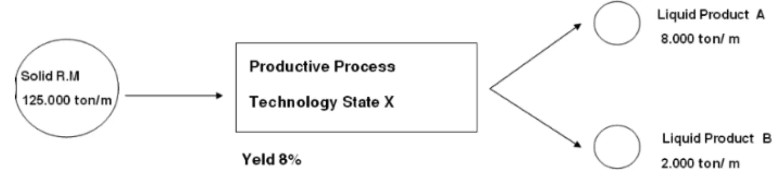
The current technological stage of the production process allows the processing of a solid gross material load of 125,000 tones (1000 kg)/month, with a yield of approximately 8% (approxi-mately 10,000 tones/month of final net product), in the proportion of 80% of product A, and 20% of product B (Fig. 1). The Research and Development project proposed by the research department of the company aims to improve the technical efficiency of the productive process by enhancing a process simulator based on computational fluid dynamics studies.

Figure 1– Current firm technology.

(5)

621

Figure 2– R&D project intended to improve technology.

The research project was divided into 3 stages of one year each, comprising the following:

Stage 1: Survey and study of more advanced fluid dynamics mathematical models and applicabil-ity to the process variables. Creation of custom algorithms with very specific parameterizations;

Stage 2: Implementation of models to optimize the variables, creation of friendly high-resolution graphical interfaces. Execution of preliminary fluid dynamics simulations;

Stage 3: Execution of tests in pilot plant and final operational adjustments, documentation and training of technical teams involved in the process.

4.1 Technical uncertainty

According to the preliminary proposition, new mathematical models will be incorporated in the operational simulator of the main reactor so that the adjustment parameters for the physical-chemical processes that occur inside may be optimized and better monitored. This change will enable more effective interventions that will result in the expected gain in productivity and greater system reliability. Because of the uncertain nature of R&D, even at an incremental level, the improvements intended are likely to occur differently from the expectations, resulting in either better or worse final yield levels as compared to the state of technology originally intended.

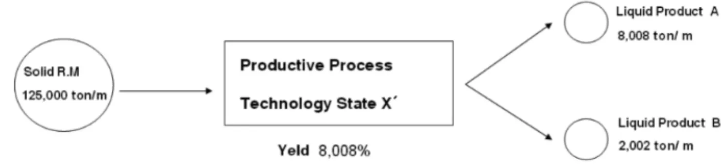
Figure 3– Firm technology at the intended state.

As the modifications to be implemented are somewhat under the control of the research group, it is possible to follow the performance of the new models at each stage. The technical uncertainty can then be endogenized and gradually “resolved”, enabling the optimal exercise of options along the development stages (Continue, Improve, Accelerate or Stop the project).

According to the preliminary expectations of the researchers, it will be possible to reach a final technology with a yield that is 0.1% superior to the current one, and higher final levels may be reached in the same way, such as 0.2%, 0.3%, and even 0.4%, according to the possibility of reaching superior technical levels upon additional investment on the project. Uncertainty

(6)

may also have a negative impact, so that it is possible to reach inferior performance levels (for example, 0.05%), or even a null or negative gain compared to the current state.

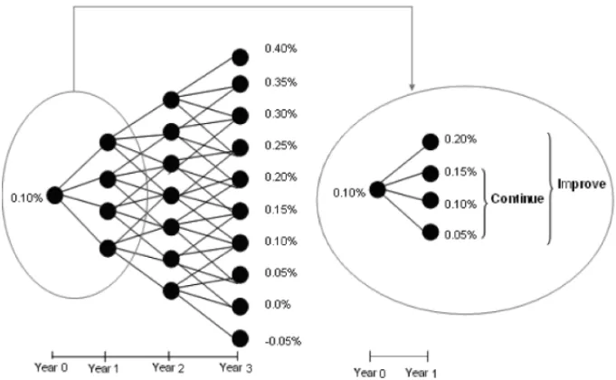
Technical variable evolution modeling, which represents the uncertainty(xt)during the

develop-ment, takes the intended level (0.1%) as its start point. At each stage, an evolution with a rate of 0.05% is applied in the case of a choice to continue, and an additional 0.05% (total of 0.1%) in the case of a choice for improvement. The resulting uncertainty tree for the technical variable in-dicates terminal knots that range from exceptional performances, such as 0.4%, to disappointing performances, such as –0.05%, according to Figure 4.

Figure 4– Uncertainty tree: transition dynamics of the level on yield gain, with focus on the possible values from gate 0 to gate 1, according to the option.

There is no precise description from assessors and researchers of the parameters that guide the evolution of the uncertainty tree. A start point that represents a feasible expectation from the researchers is assumed and, depending on the level of uncertainty of the possible final stages, the parameters that define the progression of options for continuing or improving are adjusted. In this particular case, there is a favorable asymmetry to the probable successful stages (above 0.1%), reflecting a high performance bias in the expectation of the research group. Another parameter that affects the final calculation of the value associated with each knot of the tree is the probability of success. This parameter is also guided by a strong intuitive component when it is an area of uncertainty rather than risk because the final probabilistic space connected to the survey is not well known. Based on descriptions of the uncertainty associated with the research by the researchers, this parameter was subjectively established to be 50%.

4.2 Uncertainty in development time

(7)

623

technicians, etc., is subject to variation caused by several factors. The duration of each stage of the research, therefore, will not be treated solely in a deterministic way (as it is usually treated in assessment models). Instead, the possibility of delays and advances will be assumed. Mainly as a result of technical uncertainty, R&D projects are more affected by deviations in time di-mensioning. Recognizing and treating that difficulty in the economic analysis of the project is a long-standing necessity. As mentioned above, there are two different analyses: one with deterministic time and another with stochastic time. The stochastic analysis will enable the ob-servation of the effect of a time consideration that is closer to what actually occurs during the execution of a project.

Based on the information gathered from the company, the project plan estimates its implementa-tion over the course of 3 years with a subdivision into 3 1-year stages. Just as the development may happen within a year at each stage, advances or delays relative to the time expected are pos-sible. By dividing the year into 4 quarters (which is a reasonable way to discretize the period), it is acceptable to assume that advances occur within a quarter and delays can occupy up to two quarters.

In practice, projects from the company research department are more subject to delays than advances. This delay bias is the cause of the asymmetry in the distribution, which assigns greater weight to longer times. Therefore, the uncertainty in development time has been modeled as a triangular probability distribution with its minimum value equal to 3, maximum equal to 6 and modal value equal to 4 quarter years.

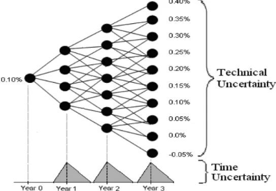
The set of three distributions for the project imposes a minimum final time of 9 quarters, or 2 years and one month, a maximum time of 18 quarters, or 4 years and 6 months, and a modal time of 12 quarters or 3 years. By dividing the time into quarters and considering the offset of a quarter produced by the accelerate option at all stages, the time dimension will consist of a total of 13 final possibilities that will form the domain of the payoff function (along with the launch performance), which will be detailed further. In a simplified view, the graphical representation of the integrated treatment of uncertainty is represented in Figure 5.

4.3 Development costs

Each stage of the research bears a typical set of costs. As a result, there is a configuration of costs associated with each consideration of the uncertainty factor “time” in the assessment of the project. Table 1 shows the distribution of these costs. Nevertheless, when time is considered in a stochastic way, it is necessary to break down the costs thoroughly in terms of the options configured, taking the fixed and variable components into account.

Generally speaking, the development costs in the deterministic model correspond to fixed costs in the stochastic model, which are added to the variable costs in the modal duration. The vari-able component of the costs in the stochastic model is directly connected to the variation of the duration estimated for each stage. In the case of the “accelerate” option in which an offset of one quarter is considered in the distribution of stage time, the magnitude of the costs associated with the exercise of such an option impacts the planning effort to advance the following stage.

(8)

Figure 5– Uncertainty tree including time uncertainty.

Table 1– Distribution of project costs by stage and option.

Stage Time treatment/ Options (amounts in US$) Type of cost Continue Improve Accelerate Stop

1

Deterministic 80,000 60,000 – –

Stochastic

Fixed 40,000 20,000 10,000 –

Variable (by Quarter) 10,000 10,000 10,000 –

2

Deterministic 120,000 80,000 – –

Stochastic

Fixed 80,000 40,000 10,000 –

3

Deterministic 200,000 100,000 – –

Stochastic

Fixed 100,000 50,000 10,000 –

Variable (by Quarter) 25,000 12.500 5,000 –

Total

Deterministic 400,000 240,000 – –

Stochastic

Fixed 220,000 110,000 30,000 –

(9)

625

4.4 Payoff curve

The payoff received from the launch of the technology is determined by the impact of its ap-plication on the gross operational cash flow of the company, as the effects of tax on additional sales of the firm are not considered. This is justified to the extent that the new technology will promote a sustainable raise of production over time with zero marginal costs. The payoff values are particularly sensitive to the project launch or implementation time. Superior values occur when the launching time of the new productive process is advanced in relation to its expected value. Therefore, inferior payoff values will occur in the case of delays.

The superior and inferior payoff values in relation to the value of the modal time were calculated by applying a fixed value of 6%, discounting the value in the case of delay, and capitalizing it in the case of advance. This approach reflects the sensitivity of the productive process to management, as the cost of opportunity is connected to that variability. The payoff values cal-culated for differing levels of efficacy consider a useful life of 5 years subsequent to the launch of the technology. Because the project is basically software that embodies new mathematical models, this depreciation period for the technology is reasonable. In the case of the determin-istic time assessment, there is a payoff value for each terminal knot, while for the stochastic case, there are 13 values corresponding to each possible final time. In the first case, there are 10 payoff values, while in the second, there are 130. Each payoff value represents an incre-mental NPV on the gross operational cash flow of the firm provoked by the new technology, in terms of additional revenues. Each value represents an additional profit because the marginal costs are zero. In this paper, risk-neutral price estimates were made for the two liquid products, types A and B, using time series models applied to their monthly historical values over 5 years (from year(−4)to year(0)).

For liquid product A, the model identified as optimal was an ARIMA(0,1,0)(differenced first-order autoregressive model), which estimated a future spot price of 0.783 US$/ton for the 12 months subsequent to the technology launch time (Fig. 12 in the attachment). In the case of product B, the optimal model was an exponential seasonal amortization, which estimated an average price of 0.736 US$/ton for the same period (Fig. 13 in the attachment). Therefore, for each level of final performance, there is the annual additional production of each product and, consequently, an annual additional profit on the cash flow once the marginal costs are zero (Table 2).

There will not be further consideration of the choice and calculation of the parameters in the time series models. We have only considered that the values estimated by those methods are long-term risk-neutral prices, which are valid for the calculation of the incremental NPV for the duration of the new technology. Also, a discount rate of 6%per annumwas adopted for this NPV, corresponding to the risk-free rate. Finally, the NPV was calculated for variations over the 5 years of operation of the new technology, which will become the payoff of each performance in the deterministic time case. The data obtained are summarized in Table 2: the annual quantity variations by product and profit (production×long-term price), the profit accrued in 5 years and

(10)

the NPV corresponding to 6% per annum. For the stochastic case, we will produce a payoff vector for each feasible final time for the project.

Table 2– Payoff in the deterministic time case.

Performance Production Profit Variation in 5 years

(%) (Ton.) (US$) (US$)

A B A B Total Profit NPV 6% p.a

0.40 384 96 300,672 70,656 371,328 1,856,640 1,444,340.00 0.35 336 84 263,088 61,824 324,912 1,624,560 1,263,790.00 0.30 288 72 225,504 52,992 278,496 1,392,480 1,083,270.00 0.25 240 60 187,920 44,160 232,080 1,160,400 902,710.00 0.20 192 48 150,336 35,328 185,664 928,320 722,150.00 0.15 144 36 112,752 26,496 139,248 696,240 541,630.00 0.10 96 24 75,168 17,664 92,832 464,160 361,080.00 0.05 48 12 37,584 8,832 46,416 232,080 180,560.00

0.00 0 0 0 0 0 0 0

–0.05 –48 –12 –37,584 –8,832 –46,416 –232,080 –180,560.00

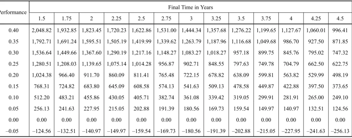
The modal time payoff corresponds to the seventh of the final stochastic times. From that value, the payoffs from previous (advanced) times will be calculated in relation to the modal time. These advanced payoff values will be greater than the modal time payoff in the same way that the payoffs from superior (deferred) times will be smaller than the modal time payoffs. The values obtained are shown in Table 3, and they are visually represented in Figure 6. The shades of gray from the payoff chart are defined according to the value as follows: Values corresponding to greater payoff are darkly shaded and values corresponding to lesser payoff are lightly shaded.

(11)

L U IS A L B E R T O ME L C H IA D E S L E IT E , JO S ´E P A U L O T E IX E IR A a n d C A R L O S P A T R ´IC IO S A MA N E Z

6

2

7

Table 3– Payoffs for stochastic time (deterministic time highlighted), in US$ 1,000.

Performance Final Time in Years

1.5 1.75 2 2.25 2.5 2.75 3 3.25 3.5 3.75 4 4.25 4.5

0.40 2,048.82 1,932.85 1,823.45 1,720.23 1,622.86 1,531.00 1,444.34 1,357.68 1,276.22 1,199.65 1,127.67 1,060.01 996.41

0.35 1,792.71 1,691.24 1,595.51 1,505.19 1,419.99 1,339.62 1,263.79 1,187.96 1,116.68 1,049.68 986.70 927.50 871.85

0.30 1,536.64 1,449.66 1,367.60 1,290.19 1,217.16 1,148.27 1,083.27 1,018.27 957.18 899.75 845.76 795.02 747.32

0.25 1,280.51 1,208.03 1,139.65 1,075.14 1,014.28 956.87 902.71 848.55 797.63 749.78 704.79 662.50 622.75

0.20 1,024.38 966.40 911.70 860.09 811.41 765.48 722.15 678.82 638.09 599.81 563.82 529.99 498.19

0.15 768.31 724.82 683.80 645.09 608.58 574.13 541.63 509.13 478.58 449.87 422.88 397.50 373.65

0.10 512.20 483.21 455.86 430.05 405.71 382.74 361.08 339.42 319.05 299.91 281.91 265.00 249.10

0.05 256.13 241.63 227.95 215.05 202.88 191.39 180.56 169.73 159.54 149.97 140.97 132.51 124.56

0.00 0.00 0.00 0.00 0.00 0.00 0.00 0.00 0.00 0.00 0.00 0.00 0.00 0.00

–0.05 –124.56 –132.51 –140.97 –149.97 –159.54 –169.73 –180.56 –191.39 –202.88 –215.05 –227.95 –241.63 –256.13

(12)

5 RESULTS FROM THE ASSESSMENT

The project has been assessed from several perspectives regarding the treatment of its main sources of uncertainty. The basic model offers an estimate of the project price by treating only the technical uncertainty, considering its development time to be fixed or deterministic and con-sidering the resulting costs in the same manner. This view coincides with the model that treats time stochastically but considersa priorithat the deadlines will be met according to the mode of the probability distribution assigned to the stage duration. The results of the deterministic (fixed duration) treatment of time will be demonstrated first by adopting the standard deterministic view, which considers 3 stages with durations of 1 year, or 4 quarters. Then, these durations are varied according to those estimated in the parameterization of the stochastic model, in terms of minimum, maximum and accelerated times. A risk-free discount rate of 6 % p.a. is considered.

5.1 Model with deterministic time

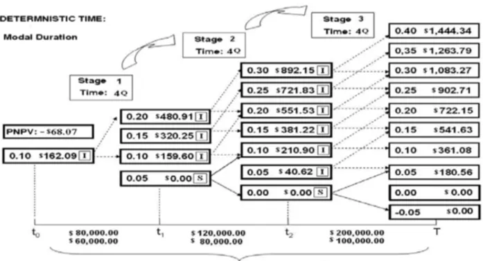
Figure 7 shows the project valuation offered by the basic model: a treatment of the technical vari-able development used by the project over a deterministic interval according to the most probvari-able outcome. A full view of the evaluation is possible, detailing the evolution of the technical un-certainty over the 3 fixed stages of a year (4 quarters or 4Q) of estimated duration, totaling 12 quarters (3 years). The uncertainty knots (represented by rectangles) introduce values of previ-ous technical performance at each stage, and their respective Active Net Present Values (ANPV, in US$ 1,000). The variable is called the ANPV to differentiate it from the Passive Net Present Value (PNPV, in US$ 1,000), which does not include any treatment of uncertainty (the value assumes that the project, once begun, will be invariably continued). The original knot, at year 0, represents the ANPV of the entire project. This is the value that will define whether the project should be started using the same basic rule of the NPV method, which instructs the initiation of a project in the case where its value is superior to 0.

(13)

629

The knots were marked with letters (within squares) that represent the optimal decision rec-ommended by the model to the project manager: “I” indicates that the optimal decision is to “improve”, “C” indicates “continue”, and “S” indicates “stop”. Dotted arrows connect the knots marked with “I” to those knots that are most likely to be reached in the following stage, while full arrows connect the others. Along the time axis, we find the listing of stage costs in US$ 1.00 associated with the choices to “continue” and “improve”; the “stop” costs are zero. This deter-ministic treatment of time does not include the option to “accelerate”. We observed that, from this viewpoint, the project is feasible under the optimal decision to “improve” att0. A projection of the probable state of the technical variable and the corresponding value of the project evolve along the tree until it reaches one of the final states that correspond to its launch at T, or imple-mentation, when it finally assumes an NPV without technical uncertainty. The value at gate 0 (the initial knot) represents the value that the implementation of the research project adds to the company. In this case, with a deterministic stage time of 1 year or 4 modal quarters of stochastic view, the amount of added value is US$ 162.09. The corresponding PNPV is –US$ 68.07, indi-cating that if the project is assumed to always “continue”, regardless of the value calculated by the technical level reached at each stage, the project would destroy company value. The PNPV defines a value for the flexibility at the rate of US$ 230.16 (US$ 162.09 – (–US$ 68.07)), and a total decision cost (in US$ 1,000.00) of US$ 140.00 (US$ 80.00+US$ 60.00).

The goal of the inclusion of model alternatives is to provide an initial evaluation that prop-erly guides the decision-making process regarding the start of the project at timet0. Along the project lifetime, new evaluations must be executed, updating the future view in terms of techni-cal development, market payoff, costs, etc., for new decision processes att1andt2. Finally, the implementation of the technological development is decided at the terminal timeT.

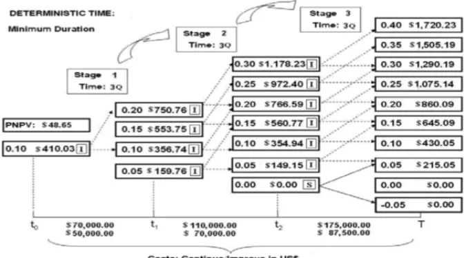
Figure 8– Evaluation of the project in the deterministic model, with fixed realization of time in the distribution minimum.

Figure 8 shows the project value (ANPV), assuming that the times indicated by the minimum levels of the frequency distributions modeled to the stochastic case would be fulfilled. This

(14)

fulfillment would produce a fixed project duration with 3 stages of 3 quarters each (0.75 year), totaling 9 quarters (2.25 years). The analysis indicates that there is a gain value associated with the variable costs not incurred in the saved quarter, as much as the payoff raised by the antici-pated time to launch or the implementation of the technology. The value for the active project (ANPV) increases from US$ 162.09 to US$ 410.03 with the reduction of one stop knot in the designed uncertainty tree. The PNPV for this time configuration, even with the probability of minimum realization under a stochastic view, is US$ 48.65. This value corroborates the conclu-sion that the reduced time allows the project to be feasible even without the active management of its technical flexibility. The value for this flexibility is now US$ 361.38, and the total decision cost is (in US$ 1,000) US$ 120.00 (US$ 70.00+US$ 50.00).

Considering the maximum duration from the deterministic viewpoint (Fig. 9), an outcome that is also unlikely in the stochastic viewpoint, the stages would last 6 fixed quarters each, totaling an 18 quarter duration of the implementation time (or 41/2years). The analysis indicates that there are value losses associated with the raise in variable costs incurred by exceeding quarters, as well as losses associated with payoff corrosion caused by a delay in the launch or implementation time for the technology. Because of the sensitivity of the values at these times, the scenario is somewhat worse in relation to the other scenarios already examined.

Figure 9– Evaluation of the project in the deterministic model, with fixed realization of time in the distribution maximum.

(15)

631

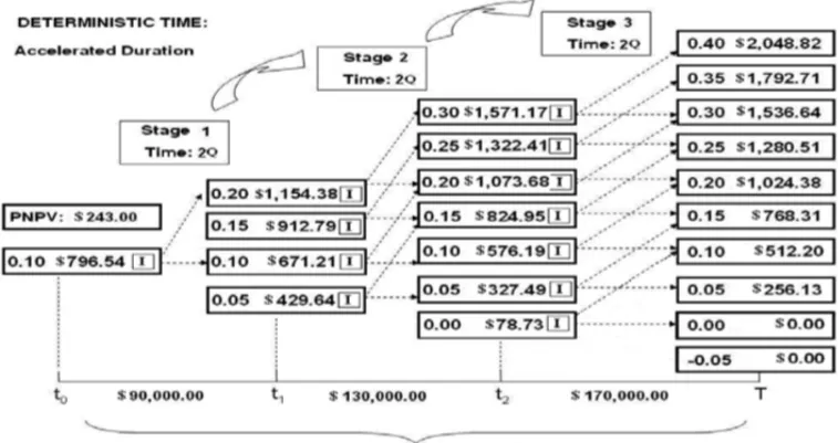
For accelerated times (Fig. 10), the project would last 3 fixed stages of 2 quarters each, totaling 6 quarters at the end of the project, or 11/2years. The outcome in this case is different from the maximum time outcome because the project gains value when time advancement allows reduced duration and higher payoff.

Therefore, the project ANPV is US$ 796.54 with a PNPV of US$ 243.00, which leads to a flex-ibility value of US$ 553.54. Objectively, these deterministic model time sensitivity exercises are an attempt to add time variability to the analysis without actually treating it in full. The most significant outcome among those analyzed is the modal time, while the minimum and max-imum time cases, treated deterministically, represent only a first approach to the full treatment offered by the stochastic time model, which will be dealt with below. The cost of the decision is US$ 90,000.00.

Figure 10– Evaluation of the project in the deterministic model, with fixed realization of time with the acceleration distribution minimum.

5.2 Model with stochastic time viewpoint

The integral model with a stochastic time treatment embodies the probability distributions that characterize the duration of the stages designed for the project in the dynamic programming algorithm. Instead of fixed durations, the model envisages 3 triangular probability distributions with the following parameters: a minimum of 3 quarters, a mode of 4 quarters and a maximum of 6 quarters (T[3;4;6]). The model also considers the use of the Monte Carlo Simulation Method and the treatment of the option to “accelerate” in the algorithm for the value calculation of the dynamic programming model.

In this case, the model is difficult to represent, and a graphical view of the project assessment as a whole makes no sense. With the large number of knots possible at each subsequent stage, the

(16)

double domain of performance versus time, and the indication of the optimal decision at each knot, a solid with the superposition of several points would be necessary, resulting in a confusing graph.

The ANPV att0in this model is US$ 405.54 (Fig. 11), with a corresponding PNPV of US$ 68.60, indicating the optimal decision for improvement, at a fixed cost of US$ 60.00. Presently, there is no exact value of the duration of stage 1 (in quarters); however, it is possible to determine the total minimum, maximum and expected costs due to this duration. According to the figures of Table 1, they are as follows:

1) Minimum: US$ 120.00 =(US$ 40.00 +3Q × US$ 10.00) +(US$ 20.00 +3Q × US$ 10.00) ;

2) Maximum: US$ 180.00= (US$ 40.00+ 6Q ×US$ 10.00) +(US$ 20.00+ 6Q × US$ 10.00) ;

3) Expected: US$ 146.80=

(US$ 40.00+4,34Q×US$ 10.00)+(US$ 20.00+4,34Q× US$ 10.00) ;

To calculate the expected cost, the mean of the triangular distribution T[3;4;6], which is ap-proximately 4.34 quarters, was used. The fixed cost of the decision is US$ 60.00 (US$ 40.00 + US$ 20.00). The flexibility value is US$ 346.94. Using this analysis route, the project seems more promising with this multiple treatment of uncertainty. The payoffs are clearly generous, awarding good performances achieved with reduced times. However, the development of a re-search project often reveals surprises held by the least interesting face of uncertainty, thus im-pairing its continuity. Prices may change, the market requirements and project costs may change, technical difficulties may arise, etc.

(17)

633

At this point, the firm intervention of a manager who makes reasonable decisions from an eco-nomic point of view makes all the difference, turning an unjustifiable loss – which often leads to filing other projects – into an acceptable loss.

In this evaluation, the project value has increased considerably relative to its value in the deter-ministic view of the modal time. The increase of the NPV is 150%, while the flexibility value increases by only 51%. This discrepancy occurs because the project value without flexibility also increases by approximately 200%, from –US$ 68.07 to US$ 58.60, which is strongly influenced by the sensitivity of the project at its implementation time.

Although these values change significantly, the optimal decision remains the same: “improve”. The results of the stochastic time model could change the decision to the additional option, “accelerate”, because the treatment of more than one source of uncertainty improves the valuation of the project, but this decision is not optimal in this case. The value gain in project flexibility is a measure of the additional information available with the adoption of a more complete model to address uncertainty, especially with a type of uncertainty that considerably affects the actual value of a project, whether it is technological or not. In the case of non-attractive evaluations, that is, very close to the acceptance limits, this model could represent a change of decision between “stop” (not starting the project) and “continue” (starting the project).

A more complete view of this set of evaluations is shown in Table 4. Among the representations of deterministic time, the most accurate model construction without a stochastic treatment of time is the one that considers the modal duration for the stochastic view (highlighted in the Table). Table 4 shows the value of flexibility associated with each optimal decision at the initial gate for project evaluation, according to the way time is addressed in the evaluation and the cost of decision.

Table 4– Summary of assessments in the two models: deterministic and stochastic times.

Time Duration Flexibility value Optimal decision Cost of decision Flex/Cost (year) (US$ 1,000.00) (US$ 1,000.00)

Deterministic:

Accelerated 1.5 US$ 553.54 Improve US$ 90.00 6.15

Minimum 2.25 US$ 361.38 Improve US$ 120.00 3.01

Modal 3 US$ 230.16 Improve US$ 140.00 1.64

Maximum 4.5 US$ 259.19 Stop US$ 0.00 –

Stochastic: T[3;4;6] US$ 346.94 Improve US$ 146.80 2.36

Although there is no change in decision in the evaluation between the deterministic-modal and stochastic models, we can improve the understanding of the quality of this decision by examining the Flexibility/Cost ratio. This value can be interpreted as the value gained by the addition of the uncertainty treatment by the unit of cost associated with the optimal decision in the project, measuring the efficiency of the decision. There is a specific cost for each possible decision.

(18)

The fixed ratio of 1.64 in the deterministic view of time increases to 2.36 in the stochastic view. Therefore, the view of the cost of a decision, adjusted for the stochastic treatment of time, resulted in a proportionally lower gain in the existing flexibility value by the unit of cost of the project. The reduction is caused by the triangular distribution used to describe the time uncertainty (the mean value is greater than the modal value).

6 CONCLUSIONS

In the example analyzed in this paper, it is possible to evaluate the evolution of value from the beginning to the end of a project from a purely deterministic treatment to a stochastic one, with broad considerations of the uncertainties that characterize the project. We can explain these different treatments by summarizing (Table 5) the main parameters adopted for each model. All models use a discounted cash flow under risk-neutral price forecasting that is discounted by a risk-free rate.

Table 5– The main parameters adopted for each model.

Model\Parameters

Research Success

Options Technical Time Costs Payoff ProbabilityP?

Available Uncertainty Uncertainty Treatment (Shape) Note:P+(1−P)=1 Treatment? Treatment?

Deterministic Model

Yes Continue No No, time constant Fixed Curve (Passive NPF Only)

Real Options Models (Active NPV)

Flexibility on Technical

Yes

Continue

Yes No, time constant Fixed by Curve

Uncertainty only Improve

Option

(Deterministic Time) Stop

Flexibility on Technical

Yes

Continue

Yes

Yes,

Fixed by Plane

Uncertainty and Improve time variable

Option +

Time Uncertainty Stop (Triangular

Variable (Stochastic Time) Accelerate Distribution)

From this comparison, it is evident that the Stochastic Time model captures more value than the others, considering the set of project data. The more complex the algorithm, the more value can be found. The main reference values (Passive or Active NPV) for each model (Deterministic or Real Options – RO) are presented in Table 6.

Table 6– The main reference values for each model.

Model Value (US$ 1,000.00) Decision

Deterministic (PNPV) –68,07 Stop

RO – Technical Uncertainty (ANPV) 162,09 Improve RO – Technical and Time Uncertainty (ANPV) 405,54 Improve

(19)

635

will also remain the same (“Stop”) in each model. Sensitivity analysis can be performed on several variables to explore the limiting values that cause a change in the optimal decision for each model. Within the same model, it is also possible that the decision does not change. For example, if the optimal option in the model of real options is “Continue”, and the PNPV is positive, the decision will be the same for the deterministic and stochastic models.

In addition to the endogenous treatment of technical uncertainty, which is certainly the most important uncertainty in a research project, the treatment of development time uncertainty pro-duces previously unsuspected values. Under a totally deterministic evaluation (both in relation to technical uncertainty and development time), the project would not be started (passive NPV of –US$ 68.07), whereas the broad treatment of its uncertainties began to add considerable value to the company (active NPV of US$ 405.54). Many successful projects end up largely exceeding their original assessments, perhaps because their flexibility value was correctly assessed, which has been previously perceived only intuitively by managers.

The application of the model proposed by Silva & Santiago (2008) to the mining firm research project showed an additional gain of 51% in flexibility value on an assessment previously ex-ecuted in a real options model without stochastic treatment of time uncertainty. The gain in flexibility value by the unit cost of the project is 44%, slightly less than because the mean value of triangular distribution T[3;4;6] it’s greater than its modal value, and, in the case of this project, more time means less value.

Certainly, a considerable portion of value is disregarded in conventional assessments; this por-tion, depending on the case, could be positive or negative. In many cases, this unconsidered value may impact decisions on the continuity of projects. The broad treatment of the main sources of uncertainty of the project is a consideration that better guides R&D portfolio composition in firms that participate in that investment category.

ACKNOWLEDGMENTS

We would like to express special gratitude for the incentive and professional support offered to this research by Lu´ıs Cl´audio de Sousa Costa and the corrections, comments and suggestions made by Reynaldo Luiz Nazareth Taylor de Lima.

REFERENCES

[1] AMRAMM & KULATILAKAN. 1999. Real Options – Managing Statregic Investment in an Uncertain World. Harvard business Scholl Press, 246 pp, Boston, MA, USA.

[2] BARROSM. 2004. Processos Estoc´asticos. Papel Virtual Editora, Rio de Janeiro.

[3] BATISTAFRS, TEIXEIRAJP, BAIDYATKN & MELOACG. 2011. Avaliação dos Métodos de Grant, Vora & Weeks e dos M´ınimos Quadrados na Determinação do Valor Incremental do Mercado de Carbono nos Projetos de Geração de Energia Elétrica no Brasil.Pesq. Oper.[online],31(1): 135–155. ISSN 0101-7438.

[4] COPELANDT & ANTIKAROVV. 2001. Real Options – A Practioner’s Guide. TEXERE, NY, USA. [5] CRESPOCFS. 2008. Avaliação do Impacto Econômico de um projeto de Pesquisa e Desenvolvimento

no valor de uma planta Gas-to-Liquids usando a Teoria das Opç ões Reais. Tese de Doutorado em Engenharia de Produção – Pontif´ıcia Universidade Cat ólica do Rio de Janeiro, Rio de Janeiro.

(20)

[6] DIXIT AK & PINDYCK RS. 1994. Investment under Uncertainty. Princeton University Press, Princeton, N.J., USA.

[7] FAULKNER TW. 1996. Applying “Option Thinking” To R&D Valuation. Research Technology Management, 39, 3 ABI/INFORM Global pg. 50.

[8] HASENCLEVERL & KUPFER D. 2002. Economia Industrial, Fundamentos Te ´oricos e Pr´aticas no Brasil. Campus, Rio de Janeiro, Brasil.

[9] HUCHZERMEIERA & LOCHCH. 2001. Project management under risk: Using real options approach to evaluate flexibility in R&D.Management Science,47: 85–101.

[10] MEDINAHV & NAVEIRORM. 1998. Materiais Avanc¸ados: Novos Produtos e Novos Processos na Ind´ustria Automobil´ıstica.Prod.,8(1): 29–44. ISSN 0103-6513.

[11] MUNJ. 2006. Real options Analysis – Tools and Techniques for Valuing Strategic Investments and Decisions. John Wiley & Sons Inc., Hoboken, New Jersey, USA.

[12] NOVAESAGNS & SOUZAJC. 2005. A Real Options Approach to a Classical Capacity Expansion Problem.Pesq. Oper.,25(2): 159–181. ISSN 0101-7438.

[13] NEVES C. 1992. Avaliação de um Investimento em Pesquisa Adicional num Novo Processo de Produção: Considerações Metodológicas e uma Aplicação.Prod.,2(2): 145–155. ISSN 0103-6513. [14] PAXONDA. 2003. Real R&D Options. Butterworth-Heinemann (Elsevier Science), Burlington, MA,

USA.

[15] ROUSSEL P, SAADKN & BOHLIN N. 1992. Pesquisa & Desenvolvimento, Como Integrar P&D ao Plano Estrat´egico e Operacional das Empresas Como Fator de Produtividade e Competitividade. Makron Books, S˜ao Paulo.

[16] SAMANEZCP. 2007. Gestão de Investimentos e Geração de Valor. Pearson Prentice Hall, São Paulo, Brasil.

[17] SANTIAGOLP & BIFANOTG. 2005. Management of R&D projects under uncertainty: A multidi-mensional approach to managerial flexibility.IEEE Transactions on Engineering Management,52: 269–280.

[18] SANTIAGOLP & VAKILIP. 2005. On the Value of Flexibility in R&D Projects.Management Science,

51: 1206–1218.

[19] SANTOSEM & PAMPLONAE. 2002. Teoria das Opções Reais: A Aplicação em Pesquisa e Desen-volvimento (P&D). Segundo Encontro Brasileiro de Finanças, IBMEC, Rio de Janeiro.

[20] SILVA TAO & SANTIAGO LP. 2009. New Product Development Projects Evaluation Under Time Uncertainty.Pesq. Oper.,29(3): 517–532. ISSN 0101-7438.

[21] SCHWARTZES. 2001. Patents and R&D as Real Options. Anderson School at UCLA. Los Angeles, CA, USA.

[22] SOUZA RC & CAMARGOME. 2004. Análise e Previsão de Séries Temporais. Gráfica e Editora Regional. Rio de Janeiro.

(21)

637

A APPENDIX

A.1 The model with deterministic time

The assessment is made along a management process that is divided into three stages (each stage corresponds to a fixed period of time), where three types of options on the project are considered: continue, improve, or abandon (stop the project). Considering a project started at t = 0 and launched onto the market at stageT, there are revision points during its development at stages t=1, . . . ,T −1.

In each of these stages, the decision taker has the flexibility to make optimal decisions regarding the project. At the following stage, t +1, the performance status of the project depends on the performance status at staget(Xt); the managerial decision(Ut); an offset (K(U t), where

K(continue) = 0 and K(improve) = 1); and the uncertainty represented byωt, a random variable

with an average of 0 and constant variance. Therefore,Xt+1may be represented as follows:

Xt+1=

(

Xt+k(ut)+ωt, if ut =Continue, Improve

Stop, if ut =Abandon

This equation will define the evolution of a multinomial tree representing the possibilities of the technological development process. In other words, it will reflect the transition dynamics of the technological variable. The development cost of each stage depends on the managerial decision. That cost is defined as follows:

c(ut)=

  

 

0, if ut =Abandon

c(t) , if ut =Continue

c(t)+α(t) , if ut =Improve

In order to begin the project activities, it is necessary to have an initial investment I, incurred att = 0. At the end of the project (at T), the performance status of the product is X, and the random market payment function is represented by 5(x). In the case where the product developed exceeds the requirements of the consumer (D), the market payoff (payment) will reach a valueM. If the product does not reach such requirements, it receives a payoff of value m. D is modeled according to a probability distribution, which has average μ and standard deviationσ.

5(X)= (

M,with prob. F(X)

m,with prob. 1−F(X)

whereF(X)=P(D<X).

Therefore, the formulation of value for each of the knots in each technology development stage is:

Vt(Xt)=max ut

−ct(ut)+

1 1+rt

E

Vt+1 Xt+1(x,ut, ωt)

fort =T,VT(Xt)=E[5(x)] ·rt =discount rate.

(22)

Figure 12– Model prepared to estimate the price of product A.

(23)

639

For the incremental R&D projects, especially those aiming at marginal efficacy improvements, the payoff curve is easily determined by a sensitivity discounted cash flow analysis of the project on the technological variable affected by the project. The result of such sensitivity is often a linear payoff curve because of the absence of scaled gains in incremental variation bands and the fact that cash flow assessment models generally use linear functions. In Figure 14, the payoff displayed follows the behavior of a normal distribution of the final performance of the technology(Xt).

Figure 14– Transition dynamics, development costs and market payoff.

In order to calculate the flexibility value, it is necessary to define the difference between active and passive management. To evaluate the passive management value, no considerations are made on the option to abandon or to improve the project at a given stage(t)(only continue is selected). This value is equivalent to the project NPV calculated att =0. Thus, the Flexibility Value= Value of Active Management – NPV.

A.2 Introducing the stochastic time

This evolution of the model is detailed in Silva & Santiago (2008) and considers a final return in the valuation of the project that now depends on both the level of development achieved and the moment of implementation of the technology or commercialization of the product. The return of the project is obtained at an uncertain future stage. Then, the option to “accelerate” the development is introduced.

At each revision stage j(j = 0, . . . ,N), the project will be characterized by a development status represented byyj =(xj,tj), wherexj is the level of development expected at the end of

the project after the execution of its first jsteps, andtj is the revision time instant. The option to

accelerate arises naturally from the stochastic treatment at each stage. In the transition dynamics, the subsequent status will be a function of the current status plus the uncertainties, both in the

(24)

development level and in duration of the step, namedξi. Therefore, Yj+1 = ϕ(Yj,uj, ξj), as

follows:

Yj+1=

                            

Stop, if uj =abandon

Yj+

ωj

tj

!

, if ut =continue

Yj+

Ij+ωj

tj

!

, if ut =improve

Yj+

ωj

tj−Aj

!

, if ut =accelerate

In the equation above,εj =(ωj,tj+1)t, whereωj is the random variable (r.v.) that represents

the technical uncertainty, andtj+1is an r.v. that represents the duration of the next step defined by the Monte Carlo simulation in the calculation algorithm represented below. At each stage of the revision j, the time will betj =P_kj₌−₁1tk, wheretk(k−1, . . . ,N)are independent r.v.s,

Ij is a constant that represents the increment of the option to “improve”, and Aj represents

a reduction in the expected duration of each step. The project payoff function is then given by 5(yN) = 5(xN,tN). For a giventn = T, the payoff function5(xN,T)is regarded as

ascending inxNand, for each performance level reached at the end of the project(xn=X), the

payoff function5(xN,tN)will usually descend with the postponing of launch time because of

the incomplete fulfillment of the market needs at a delayed launch time. The development costs are then represented by:

CkYj,uj,tk =

              

0, if uj =abandon

Kk(tk,uj) , if ut =continue

Kk(tk,uj)+αk, if ut =improve

Kk(tk,uj)+βk, if ut =accelerate

The dynamic programming model can be described as follows: Let Gj(yj,uj) be the value

function expected when the controluj is applied, at stateyj. These (uj andyj) are represented

as follows:

G(Yj,uj)=

(

0, uj =Abandon

Etj

Eωj|tj

−Cj+1(Yj,uj,tj+1)+Vj+1(Yj+1)

tj, Otherwise

In the equation above,Vj+1represents the project value at decision stage j+1 and is assessed as follows:

Vj(yj)=max uj∈2

(25)

641

2is the set of controls available (2 = {Abandon, Continue, Improve, accelerate}). Finally, by incorporating the boundary condition of the commercialization time, Vn(yn)= 5(yn), the

dynamic programming model can be written as:

Objective:V0

s.a.:Vn(Yn)=5(Yn)

Vj(yj)=max uj∈2

Gj(yj,uj)

With the introduction of stochastic time, it is no longer possible to generate a simplified graphical view of the project as a whole, as shown in Figure 14; however, it is possible to produce a simple graphic visualization of what may occur at the subsequent stage, as shown in Figure 15.

Figure 15– Graphic view of the knots likely to be reached at the subsequent stage.