ABSTRACT: In order to make a sensible prediction on the air trafic low management with conditions of wave-off and bolter, a system dynamic model for the night recovery operations of embarked aircrafts is built to ensure the adaption of air trafic low with the capacity of air control at each phase of the recovery operations. The model aims at the characteristics of multiple feedbacks, delays and complex time varying, builds a stock low diagram and operation model with impact factors of the night recovery system, and is simulated in Vensim® Personal Learning Edition 5.9. The simulation shows a reasonable prediction result for the night recovery of embarked aircrafts with conditions of bolter and wave-off and can provide a theoretical basis for scheduling the air trafic low management of embarked aircrafts formation recovery.
KEYWORDS: Air trafic low management, Recovery, Embarked aircrafts formation, System dynamics, Complex system modeling.
A Prediction Model for Night Recovery of
Embarked Aircrafts Based on System Dynamics
Liangliang Cheng1,3, Kuizhi Yue1,2, Zhenghao Huang2
INTRODUCTION
Aircraft Carrier Attack (CVA), with the ability of fast oversea power projection, becomes the main combat force of modern navies. For a large number of aircrats in the process of formation recovery, secure, efficient and sequential air traic low managements are necessary to make full use of the capacity of airspace and light deck, improve the utilization of time and space, and provide the latest information for the carrier-aircrats system.
The issue on civil air traffic flow management has been well studied by researchers both at home and abroad. Taking the complexity of the air traffic management system (Zhang et al. 2009) into consideration, researchers presented 3 approaches to solve the air traffic flow management problem: air traffic capacity management (Yang and Hu 2010), ground holding management (Ye and Hu 2010) and flight schedule optimization (Zhang and Hu 2010). Meng et al. (2012) studied the problem of air traffic flow management in uncertain severe convective weather and established a dynamic reroute planning model based on genetic algorithms. In Liu and Hu (2011), an auction-based market method was proposed to solve the congestion problem of airspace in the stage of pre-tactic and tactic air traffic flow management, and a decision-making model for airline company was analyzed based on game theory. Bertsimas
et al. (2008) used an integer optimization method to research the air traffic flow management while DeArmo et al. (2010) studied the preliminary benefits of the analysis of air traffic flow management. Weigang et al. (2008) studied a decision-support system of the tactical air traffic flow management.
1.Beijing University of Aeronautics and Astronautics – School of Aeronautic Science and Engineering – Department of Aircraft Design – Beijing – China.2.Naval Aeronautical University – Department of Airborne Vehicle Engineering – Staff Room of Aircraft – Yantai/Shandong – China. 3.Naval Aeronautical University – Department of Carrier-Based Engineering – Aviation Maintenance Teaching Group – Huludao/Liaoning – China.
Author for correspondence: Kuizhi Yue | Naval Aeronautical University – Department of Airborne Vehicle Engineering – Staff Room of Aircraft | 188 Erma Road |
A dynamic model for air traffic flow management and a research about the flight deck scheduling based on distributed network were presented in Mukherjee and Hansen (2009) and Dastidar and Frazzoli (2011), respectively. Ryan et al. (2011) designed an interactively local and global decision-support system for aircraft carrier deck scheduling. In Yue et al.
(2013a), the stock flowchart and the mathematical model of the complex time-varying system for dynamic handling of embarked aircrafts were built based on system dynamics (SD) after discussion of the process of aircraft turnaround and transferring of embarked aircrafts among the flight deck, hangar and elevators. In Yue et al. (2013b), to make a reasonable schedule of recovery considering wave-off and bolter of aircrafts, an operation model on embarked aircraft recovery in good weather was built. Wesonga (2015) presented a practical stochastic optimization model for air traffic flow management (ATFM) of airports, considering the airport delay based on multivariate statistics. The uncertainty of effective measures in ATFM was estimated with multivariate probabilistic collocation method (PCM) in Zhou et al. (2014). The issue of determining the stochastic capacity of airspace in ATFM was discussed in Clarke et al. (2013). The heating effect of jet blast from 4 embarked aircrafts on take-off zone of the flight deck was studied in Yue et al. (2015a) based on CFD technique and, similarly, the impact of the jet blast on the jet blast deflector (JBD) was discussed based on CFD theory in Yue et al. (2015b).
Nevertheless, researches on the system modeling problems of ATFM model, like multiple feedback factors, time delay and complex time-varying, are not sufficient. In addition, the study on the differences of ATFM between the aircraft carrier and civil airport brought by different environments and platforms is also inadequate. For example, due to the high risk of night recovery of embarked aircrafts, an accurate recovery schedule is necessary to ensure the security. However, if bolter or wave-off happens due to landing misses, the time schedule of recovery will be disrupted, recovery will be delayed, reduction of efficiency will be consequent, and the recovery security will be even harmed.
In order to solve the existing problems in the previous models, a system dynamic method is applied in this study to build an ATFM model of embarked aircraft night recovery. It is expected that it provides a viable solution to solve such ATFM problems.
PREDICTION MODEL
System dynamics is an integrated science of systems theory and computer simulation focusing on the system feedbacks and actions (Yue et al. 2011). It is introduced into various ields, such as economic, military, and ecological to solve the problems of complex non-linear giant systems with feedback structures (Wolstenholme 2003; hompson and Tebbens 2007).
The prediction model based on system dynamics theory has 4 parts: the analysis of night recovery process of embarked aircraft formation, the system boundaries determination and basic assumptions, stock flow diagram analysis and equation setups.
NIGHT RECOVERY PROCESS OF EMBARKED AIRCRAFT FORMATION ANALYSIS
Night recovery of embarked aircrat is quite diferent from that in the daytime, because this operates under the Case I weather condition while night recovery is conducted under the Case III one.
he process of night recovery of embarked aircrat forma- tion includes the arrival, approach, final approach, deck landing, bolter or wave-of phases (Figs. 1 and 2).
Wave-of means the maneuver of nose-up for climbing of the embarked aircrat before touching the deck. It happens generally in adverse meteorological conditions of landing, inappropriate manipulating of the pilot, excessive deck motion etc. Bolter happens if the tail hook of the aircrat bouncing above the arrestor cable when touching the deck or the aircrat misses all the cables on the arresting area when landing. In this case, the aircrat must be powered up immediately to climb for safety.
Figure 1. Flight cross-sectional view of the night recovery of embarked aircraft formation.
D
E
B
C A
1,000 2,000
–10 0 10 20 30 40 50 60 70 80 90 100 h/m
THE DETERMINATION OF SYSTEM BOUNDARIES AND BASIC ASSUMPTIONS
The system boundaries of the prediction model depend primarily on the scope and span of the variables and time, being determined according to the state variables. The subject of this paper is the number of embarked aircrafts at each phase of the night recovery. Only the related entities are concerned, including the number of embarked aircrafts at the mentioned phases (A — arrival; B — approach; C — final approach; D — deck landing; E — bolter or wave-off; Fig. 1), deck arrestor gear area, flight deck landing area and temporary spots. The connections of the entities form the entire system discussed here.
Various uncertainties exist in the night recovery process during over-sea operations. The primary concerns of this research include key factors such as spinning of the embarked aircrafts, target acquisition with landing director radar and optical landing aid system, wave-off, bolter, touching the deck, arresting, and taxiing.
he following assumptions are presented to simplify the prediction system:
• he night recovery system of embarked aircrats is continuous over time.
• he remaining fuel of aircrats is suicient for landing, waving-of and bolter.
• Flight accidents are excluded from the model.
Figure 2. Vertical view of night recovery patterns for embarked aircrafts.
Bolter or wave-off phase
Deck landing phase Final approach phase
Approach phase 20 km
24 km
38 km
40 km
100 km
Arrival phase
STOCK FLOW DIAGRAM ANALYSIS
The stock flow diagram is built to distinguish the variables, clarify the logical relationships among the various elements, feedback forms and control laws of the system. It is a representation method with intuitive symbols for further research on the system.
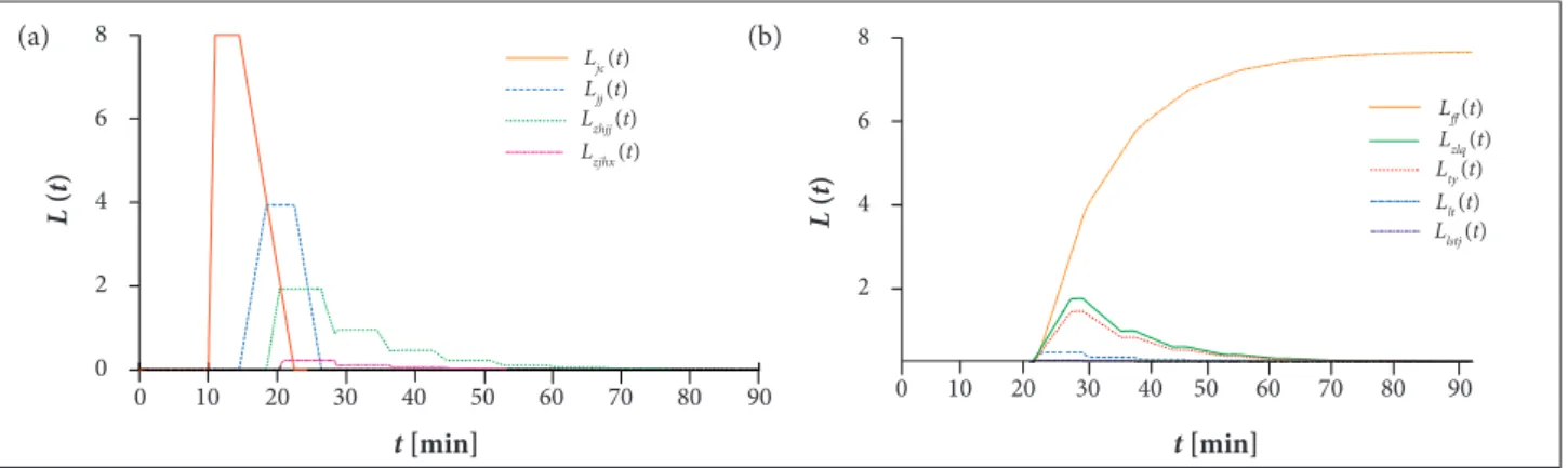
The stock flow diagram of the prediction system is a structural description of the arrival holding pattern, approach and inal approach, landing route, wave-of, bolter, arresting gear area, deck landing area and temporary spots. It holds much more information than written statements can do and is clearer and more accurate in logic. he diagram consists of 9 state variables, 11 rate variables and 23 auxiliary variables (Fig. 3).
EQUATION ESTABLISHMENT
he operation of the prediction system has the characte- ristics of complex time-varying. Figure 3 presents the explana- tions of the system, which can improve the understanding of Eqs. 1 to 24.
(1)
(2)
(3)
(4)
(5)
(6)
(7)
(8)
(9)
) ( ) ( ) (
t t
dt t dL
tcdd jc
jc
ξ
ξ
−=
ξ
ξ −
ξ
ξ
ξ
ξ
−ξ
ξ
ξ
− −ξ
ξ −
ξ
ξ
ξ
− −ξ
ξ −
ξ
ξ −
ξ
ξ
ξ
−) ( ) ( ) (
t t dt
t dL
ld tcdd jj
ξ
ξ −
=
ξ
ξ
ξ
ξ
−ξ
ξ
ξ
− −ξ
ξ −
ξ
ξ
ξ
− −ξ
ξ −
ξ
ξ −
ξ
ξ
ξ
−ξ
ξ −
) ( ) ( ) ( ) ( ) (
t t t
t dt
t dL
g tyq ffq
ld zhjj
ξ
ξ
ξ
ξ
+ + −=
ξ
ξ
ξ
− −ξ
ξ −
ξ
ξ
ξ
− −ξ
ξ −
ξ
ξ −
ξ
ξ
ξ
−ξ
ξ −
ξ
ξ
ξ
ξ
−) ( ) ( ) ( ) (
t t t dt
t dL
cj j
ξ
ξ
ξ
− −=
ξ
ξ −
ξ
ξ
ξ
− −ξ
ξ −
ξ
ξ −
ξ
ξ
ξ
−ξ
ξ −
ξ
ξ
ξ
ξ
−ξ
ξ
ξ
− −) ( ) ( ) (
t t
dt t dL
r
ξ
ξ −
=
ξ
ξ
ξ
− −ξ
ξ −
ξ
ξ −
ξ
ξ
ξ
−ξ
ξ −
ξ
ξ
ξ
ξ
−ξ
ξ
ξ
− −ξ
ξ −
) ( ) ( ) ( ) (
t t t dt
t dL
t cj l
ξ
ξ
ξ
− −=
ξ
ξ −
ξ
ξ −
ξ
ξ
ξ
−ξ
ξ −
ξ
ξ
ξ
ξ
−ξ
ξ
ξ
− −ξ
ξ −
ξ
ξ
ξ
− −) ( ) ( ) (
t t
dt t dL
t
ξ
ξ −
=
ξ
ξ −
ξ
ξ
ξ
−ξ
ξ −
ξ
ξ
ξ
ξ
−ξ
ξ
ξ
− −ξ
ξ −
ξ
ξ
ξ
− −ξ
ξ −
) ( ) ( ) (
t t dt
t dLlt
ξ
ξ −
=
ξ
ξ
ξ
−ξ
ξ −
ξ
ξ
ξ
ξ
−ξ
ξ
ξ
− −ξ
ξ −
ξ
ξ
ξ
− −ξ
ξ −
ξ
ξ −
) ( ) (
t dt
t dL
tj
ξ
where: Ljc(t) is the number of embarked aircrafts in arrival holding pattern; t represents time, in min; ξjc(t) is the flow rate of arriving embarked aircrafts; ξtcdd(t) is the flow of embarked aircrafts departing from the spin holding pattern; Ljj(t) is the number of aircrafts in approach phase; ξld(t) is the flow rate of embarked aircrafts captured by landing director radar; Lzhjj(t) is the number of embarked aircrafts in final approach; ξffqr(t) is the flow rate of embarked aircrafts from wave-off
to final approach; ξtyqr(t) is the flow rate of aircrafts from bolter to final approach; ξgx(t) is the flow rate of embarked aircrafts captured by optical landing aid system; Lzjhx(t) is the number of embarked aircrafts deck in landing pattern; ξff(t) is the flow rate of embarked aircrafts waving off; ξcj(t) is the flow rate of embarked aircrafts touching the flight deck; Lff(t) is the number of embarked aircrafts waving off; Lzlq(t) is the number of embarked aircrafts in the arresting gear area;
Figure 3. Stock low diagram of the prediction system for the night recovery of embarked aircrafts.
Number of embarked aircrafts in the arresting gear area
Number of embarked aircrafts on temporary aircraft spots Flow rate of
embarked aircrafts arrested Number of aircrafts
at approach phase
Number of embarked aircrafts bolting Flow rate of aircrafts
from bolter to final approach
Number of embarked aircrafts at final approach Flow rate of embarked
aircrafts captured by landing director radar
Number of embarked aircrafts deck in landing pattern
Flow rate of embarked aircrafts touching the
flight deck Flow rate of embarked
aircrafts captured by optical landing aid system
Number of embarked aircrafts in arrival holding pattern
Flow rate of arriving embarked aircrafts Flow of embarked aircrafts departing from the spin holding pattern
Number of embarked aircrafts waving-off
Flow rate of embarked aircrafts
waving-off Flow rate of embarked
aircrafts from wave-off to final approach
Number of embarked aircrafts in deck landing area
Flow rate of embarked aircrafts
taxing on deck Flow rate of
embarked aircrafts bolting
Probability of wave-off
Probability of bolter
Time of taxiing for each aircraft Arrested time Time of bolter
Time from bolter to final approach
Time from landing to touching the flight deck Distance of the landing pattern
Landing speed Time from wave-off
to final approach
Time in which a wave-off occurs
Capture time Distance at final
approach phase
Final approaching speed of embarked aircrafts Distance at approach phase
Approaching speed Time of radar capture
Distance at arrival phase
Arrival speed Delay time
Arrival time
Number of recovering embarked aircrafts
Expected number of embarked aircrafts in
ξzl(t) is the flow rate of embarked aircrafts arrested; ξty(t) is the flow rate of embarked aircrafts bolting; Lty(t) is the number of embarked aircrafts bolting; Llt(t) is the number of embarked aircrafts in deck landing area; ξhx(t) is the flow rate of embarked aircrafts taxing on deck; Llstj(t) is the number of embarked aircrafts on temporary aircraft spots.
(10) (13) (15) (17) (24) (18) (11) (12) (14) (16) (19) (20) (21) (22) (23)
where: mhs is the number of recovering embarked aircrats; tjc is the arrival time, in min; PULSE(tjc,1) is the single impulse function with a start point tjc and a length of 1; tyc is the delay time, in min; ndb is the expected number of embarked aircrats in each batch; ljcis the distance in arrival phase, in m; vjcis the arrival speed, in m/min; ηgd(.,.,.) is the pipeline delay function; tld is the time of radar capture, in min; ljj is the distance in approach phase, in m; vjj is the approaching speed, in m/min; tbh is the capture time, in min; lzhjj is the distance in inal approach phase, in m; vzhjj is the inal approaching speed of embarked aircrats, in m/min; tffqr is the time from wave-of to inal approach, in min; ttyqr is the time from bolter to inal approach, in min; ξff is the probability of wave-of; txhff is the time when a wave-of occurs, in min; txhcj is the time from landing to touching the light deck, in min; lzjhx is the distance of the landing pattern, in m; vzjhx is the landing speed, in m/ min; λty is the probability of bolter; tty is the time of bolter, in min; tzl is the arrested time, in min; thx is the time of taxiing for each aircrat, in min.
SIMULATION CASES AND ANALYSIS
he model according to Eqs. 1 – 24 were simulated in Vensim® Personal Learning Edition 5.9. In this section, the model of night recovery is simulated based on the Russian aircrat carrier Kuznetsov. he initial values of the factors of the prediction system are: Ljc(t0) = 0, Ljj(t0) = 0, Lzhjj(t0) = 0, Lzjhx(t0) = 0, Lff(t0) = 0, Lzlq(t0) = 0, Llt(t0) = 0, Llstj(t0) = 0, mhs = 8, tjc = 10 min, ndb = 8, ljc = 60 km, vjc = 800 km/h, ljj = 25 km, vjj = 380 km/h, lzhjj = 9 km, vzhjj = 280 km/h, tfqr = 6 min, ttyqr = 6 min, λf = 0.2, txhf = 10 s, lzjhx = 1 km, vzjhx = 240 km/h, λty = 0.3, tty = 3 s, tzl = 3 s and thx = 30 s. he control parameter t = 0 ~ 90 min.
WAVE-OFF OR BOLTER
The mathematical model of night recovery is a non-linear time-varying complex giant system with delays and feedback loops. The probability of wave-off and bolter is relatively high in night recovery. he simulation results of the number of aircrats at each stage of the night recovery for an 8-aircrat formation with λf = 0.2 and λty = 0.3 are shown in Fig. 4.
In Figs. 4 and 5, the abscissa represents the time points of the embarked aircrats in the recovery process and the vertical axis represents the quantity of embarked aircrats.
) 1
,
( )
( hs jc
jc t =m ×PULSE t
ξ
≥ ξ
ξ
η
ξ
l ξ ξ ξ η ξ ξ η ξ ξ η ξ × ≥ 0 ) ( 0 0 ) ( / ) ( ) ( t L t L t t L t zjhx zjhx xhff ff zjhx ff λ ξ × − ≥ 0 ) ( 0 0 ) ( / ) 1 ( ) ( ) ( t L t L t t L t zjhx zjhx xhcj ff zjhx cj λ ξ zjhx zjhx xhcjv
l
t
×λ ≥
ξ
× −λ ≥
ξ
ξ
×ξ
< ≥ + = 0 ) ( 0 0 ) ( ) ( ) ( t L t L n t t PULSE t jc jc db yc jc tcdd ξξ
η
ξ
l ξ ξ ξ η ξ ξ η ξ ξ η ξ × ≥ 0 ) ( 0 0 ) ( / ) ( ) ( t L t L t t L t zjhx zjhx xhff ff zjhx ff λ ξ × − ≥ 0 ) ( 0 0 ) ( / ) 1 ( ) ( ) ( t L t L t t L t zjhx zjhx xhcj ff zjhx cj λ ξ zjhx zjhx xhcjv
l
t
×λ ≥
ξ
× −λ ≥
ξ
ξ
×ξ
≥ ξ jc jc yc v l t =ξ
η
ξ
l ξ ξ ξ η ξ ξ η ξ ξ η ξ × ≥ 0 ) ( 0 0 ) ( / ) ( ) ( t L t L t t L t zjhx zjhx xhff ff zjhx ff λ ξ × − ≥ 0 ) ( 0 0 ) ( / ) 1 ( ) ( ) ( t L t L t t L t zjhx zjhx xhcj ff zjhx cj λ ξ zjhx zjhx xhcjv
l
t
×λ ≥
ξ
× −λ ≥
ξ
ξ
×ξ
≥ ξ ) ( )( tcdd ld
ld t
η
ξ
t tξ
=l ξ ξ ξ η ξ ξ η ξ ξ η ξ × ≥ 0 ) ( 0 0 ) ( / ) ( ) ( t L t L t t L t zjhx zjhx xhff ff zjhx ff λ ξ × − ≥ 0 ) ( 0 0 ) ( / ) 1 ( ) ( ) ( t L t L t t L t zjhx zjhx xhcj ff zjhx cj λ ξ zjhx zjhx xhcj
v
l
t
×λ ≥
ξ
× −λ ≥
ξ
ξ
×ξ
≥ ξξ
η
ξ
jj jj ld l t =ξ ξ ξ η ξ ξ η ξ ξ η ξ × ≥ 0 ) ( 0 0 ) ( / ) ( ) ( t L t L t t L t zjhx zjhx xhff ff zjhx ff λ ξ × − ≥ 0 ) ( 0 0 ) ( / ) 1 ( ) ( ) ( t L t L t t L t zjhx zjhx xhcj ff zjhx cj λ ξ zjhx zjhx xhcj
v
l
t
×λ ≥
ξ
× −λ ≥
ξ
ξ
×ξ
≥ ξξ
η
ξ
( ) ( ) ( ) ( b !t"# $ %%# $ ld & ' & ( t t t t
t η ξ ξ ξ
ξ = + +
ξ η ξ ξ η ξ × ≥ 0 ) ( 0 0 ) ( / ) ( ) ( t L t L t t L t zjhx zjhx xhff ff zjhx ff λ ξ × − ≥ 0 ) ( 0 0 ) ( / ) 1 ( ) ( ) ( t L t L t t L t zjhx zjhx xhcj ff zjhx cj λ ξ zjhx zjhx xhcj
v
l
t
×λ ≥
ξ
× −λ ≥
ξ
ξ
×ξ
≥ ξξ
η
ξ
ξ ξ ξ η ξ *+jj * +jj -+ . l t =ξ η ξ ξ η ξ × ≥ 0 ) ( 0 0 ) ( / ) ( ) ( t L t L t t L t zjhx zjhx xhff ff zjhx ff λ ξ × − ≥ 0 ) ( 0 0 ) ( / ) 1 ( ) ( ) ( t L t L t t L t zjhx zjhx xhcj ff zjhx cj λ ξ zjhx zjhx xhcj
v
l
t
×λ ≥
ξ
× −λ ≥
ξ
ξ
×ξ
≥ ξξ
η
ξ
ξ ξ ξ η ξ / 1 21 ( )( 6 7 33 3345
3345 t η ξ t t
ξ =
ξ η ξ
× ≥ 0 ) ( 0 0 ) ( / ) ( ) ( t L t L t t L t zjhx zjhx xhff ff zjhx ff λ ξ × − ≥ 0 ) ( 0 0 ) ( / ) 1 ( ) ( ) ( t L t L t t L t zjhx zjhx xhcj ff zjhx cj λ ξ zjhx zjhx xhcj
v
l
t
×λ ≥
ξ
× −λ ≥
ξ
ξ
×ξ
≥ ξξ
η
ξ
ξ ξ ξ η ξ ξ η ξ 8 9 :9 ( ) ( t ;< = ty >?t;< =
t t
t η ξ
ξ =
× ≥ 0 ) ( 0 0 ) ( / ) ( ) ( t L t L t t L t zjhx zjhx xhff ff zjhx ff λ ξ × − ≥ 0 ) ( 0 0 ) ( / ) 1 ( ) ( ) ( t L t L t t L t zjhx zjhx xhcj ff zjhx cj λ ξ zjhx zjhx xhcj
v
l
t
×λ ≥
ξ
× −λ ≥
ξ
ξ
×ξ
≥ ξξ
η
ξ
ξ ξ ξ η ξ ξ η ξ ξ η ξ < ≥ × = 0 ) ( 0 0 ) ( / ) ( ) ( t L t L t t L t zjhx zjhx xhff ff zjhx ff λ ξ × − ≥ 0 ) ( 0 0 ) ( / ) 1 ( ) ( ) ( t L t L t t L t zjhx zjhx xhcj ff zjhx cj λ ξ zjhx zjhx xhcj
v
l
t
×λ ≥
ξ
× −λ ≥
ξ
ξ
×ξ
≥ ξξ
η
ξ
ξ ξ ξ η ξ ξ η ξ ξ η ξ × ≥ 0 ) ( 0 0 ) ( / ) ( ) ( t L t L t t L t zjhx zjhx xhff ff zjhx ff λ ξ < ≥ − × = 0 ) ( 0 0 ) ( / ) 1 ( ) ( ) ( t L t L t t L t zjhx zjhx xhcj ff zjhx cj λ ξ zjhx zjhx xhcjv
l
t
×λ ≥
ξ
× −λ ≥
ξ
ξ
×ξ
≥ ξξ
η
ξ
ξ ξ ξ η ξ ξ η ξ ξ η ξ × ≥ 0 ) ( 0 0 ) ( / ) ( ) ( t L t L t t L t zjhx zjhx xhff ff zjhx ff λ ξ × − ≥ 0 ) ( 0 0 ) ( / ) 1 ( ) ( ) ( t L t L t t L t zjhx zjhx xhcj ff zjhx cj λ ξ zjhx zjhx xhcjv
l
t
=
×λ ≥
ξ
× −λ ≥
ξ
ξ
×ξ
≥ ξξ
η
ξ
ξ ξ ξ η ξ ξ η ξ ξ η ξ × ≥ 0 ) ( 0 0 ) ( / ) ( ) ( t L t L t t L t zjhx zjhx xhff ff zjhx ff λ ξ × − ≥ 0 ) ( 0 0 ) ( / ) 1 ( ) ( ) ( t L t L t t L t zjhx zjhx xhcj ff zjhx cj λ ξ zjhx zjhx xhcjv
l
t
< ≥ × = @ ) ( @ @ ) ( A ) ( ) ( t L t L t t L t B CD B CD ty ty BCD ty λ ξ
× −λ ≥
ξ
ξ
×ξ
≥ ξξ
η
ξ
ξ ξ ξ η ξ ξ η ξ ξ η ξ × ≥ 0 ) ( 0 0 ) ( / ) ( ) ( t L t L t t L t zjhx zjhx xhff ff zjhx ff λ ξ × − ≥ 0 ) ( 0 0 ) ( / ) 1 ( ) ( ) ( t L t L t t L t zjhx zjhx xhcj ff zjhx cj λ ξ zjhx zjhx xhcjv
l
t
×λ ≥
ξ < ≥ − × = E ) ( E E ) ( F ) 1 ( ) ( ) ( t L t L t t L t GHI GHI GH ty GH I GH λ ξ
ξ
×ξ
≥ ξξ
η
ξ
ξ ξ ξ η ξ ξ η ξ ξ η ξ × ≥ 0 ) ( 0 0 ) ( / ) ( ) ( t L t L t t L t zjhx zjhx xhff ff zjhx ff λ ξ × − ≥ 0 ) ( 0 0 ) ( / ) 1 ( ) ( ) ( t L t L t t L t zjhx zjhx xhcj ff zjhx cj λ ξ zjhx zjhx xhcjv
l
t
×λ ≥
ξ
× −λ ≥
ξ
JK
lt
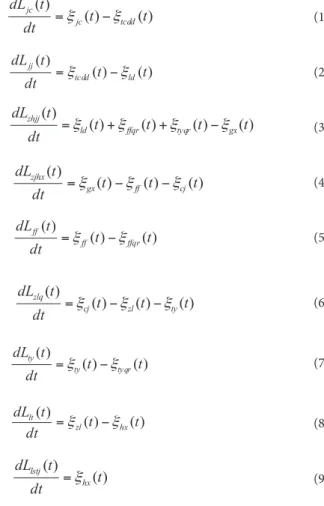
Figure 4a shows the quantity of embarked aircrafts during night recovery at the arrival, approach, final approach and landing pattern phases. At the arrival phase, embarked aircrafts are assumed to enter when t = 10 min and it is completed when t = 11 min; when t = 14.5 min, embarked aircrafts in the 8-aircraft formation begin to withdraw from spin holding pattern in turn, and the phase is finished when t = 22.5 min. The arrival phase has a range of 60 km for the spin holding pattern, and the withdrawing rate of aircrafts can be controlled at 1 aircraft per min. When t = 14.5 min, the formation of embarked aircrafts enters the approach phase in turn. For the relatively small range about 25 km for the approach stage, a maximum of 4 aircrafts can be held in this phase. When t = 18.4 min, aircrafts will be captured by landing director radar and then enter the final approach phase. The whole approach phase will be finished at t = 26.4 min. The status at this phase becomes complex — the maximum number of aircrafts can reach 2, but for the aircrafts re-entering from wave-off or bolter, the quantity
can be divided into 7 levels. The number reduces below 0.1 from t = 59.4 min. The quantity of embarked aircrafts at the landing pattern phase is also complex — the phase begins at t = 20.4 min and, for the distance of landing pattern, it is about 1 km; the aircrafts only spend 0.25 min at a speed of 240 km/h in the pattern. Then the maximum number of aircrafts is 0.25 per min. The quantity of aircrafts of this phase also has 7 levels for the same reason of wave-off and bolter. The number of aircrafts reduces below 0.01 per min from t = 61.1 min.
Figure 4b shows the quantity of embarked aircrats at each phase of the night recovery operations. he case of wave-of and bolter makes the status complex and divides the quantity of embarked aircrats into 7 levels.
Embarked aircrafts enter the temporary spots when t = 21 min; when t = 45.1 min, the quantity of embarked aircrats entering into the deck temporary spots is 7 and, when t = 64 min, that number reaches 7.8, which means that 97.5% of embarked aircrats are recovered in probability.
Figure 5. The quantity of embarked aircrafts at each stage without wave-off or bolter. (a) Embarked aircrafts before touching the light deck; (b) Embarked aircrafts after touching the light deck.
Figure 4. The quantity of embarked aircrafts at each phase in the case of wave-off or bolter. (a) Embarked aircrafts in touch before the light deck; (b) Embarked aircrafts after touching the light deck.
0
0 10 20 30 40 50 60 70 80 90
2 4 6 8
L
(
t
)
2 4 6 8
L
(
t
)
Ljc (t)
Ljj (t)
Lzhjj (t)
Lzjhx (t)
Lff (t) Lzlq (t) Lty (t) Llt (t) Llstj (t)
1 0
0 2 0 3 0 4 0 5 0 6 0 7 0 8 0 9 0
t [min] t [min]
0
0 10 20 30 40 50 60 70 80 90
2 4 6 8
L
(
t
)
2 4 6 8
L
(
t
)
Ljc (t)
Ljj (t)
Lzhjj (t)
Lzjhx (t)
Lff (t)
Lzlq (t) Lty (t) Llt (t) Llstj (t)
10
0 20 30 40 50 60 70 80 90
t [min] t [min]
(a)
(a)
(b)
WITHOUT WAVE-OFF AND BOLTER
he simulation results in the case without wave-of and bolter, which means λf = 0 and λty = 0 are shown in Fig. 5. It can be derived that, for an 8-aircrat formation, 12.5 min are spent at the arrival phase, 12 min at the approach phase, and the time spent at the inal approach, landing pattern, arrestor gear area, landing area and temporary spots are 9.875; 8; 8; 8 and 10 min, respectively.
he simulation results in both cases have a high reliability according to the capacity of ATFM of the Kuznetsov carrier during night recovery of embarked aircrat formation.
CONCLUSIONS
The prediction model of night recovery of embarked aircraft formation can provide receivable simulation results for air traffic forecasting in the case of bolter and wave-off to ensure that the flow of aircrafts at each phase of recovery is in accordance with the capacity of ATFM. The implement of air traffic schedule and flight plan can benefit from the simulation results so that delays, holding time and other bottlenecks of the recovery process will be minimized. The results can provide the theoretical and technical basis for the development and implementation of ATFM of embarked aircrafts recovery.
he following results were achieved through the research: • A sensible prediction model for night recovery of
embarked aircrat formation can be established based on the method of system dynamics.
• The characteristics of multiple feedbacks, delays, complex time varying, non-linearity and dynamics of the recovery system are well reflected in the model.
• he simulation results correspond to the case of light test of embarked aircrats.
ACKNOWLEDGEMENTS
he authors thank the National Natural Science Foundation of China.
AUTHOR’S CONTRIBUTION
Conceptualization, Yue K and Cheng L; Methodology, Yue K, Cheng L, and Huang Z; Investigation, Cheng L and Huang Z; Writing – O r i g i n a l D r af t , Yu e K an d Hu ang Z ; Wr it ing – R e v ie w & E dit ing , C heng L and Yue K; Funding Ac q u i s i t i o n , Yu e K ; R e s o u r c e s , C h e n g L a n d Hu a n g Z ; Sup er v ision, Yue K.
REFERENCES
Bertsimas D, Guglielmo L, Odoni A (2008) The air traffic flow management problem: an integer optimization approach. Proceedings of 13th International Conference; Bertinoro, Italy.
Clarke JPB, Solak S, Ren L, Vela AE (2013) Determining stochastic airspace capacity for air traffic flow management. Transport Sci 47(4):542-559. doi: 10.1287/trsc.1120.0440.
Dastidar RG, Frazzoli E (2011) A queueing network based approach to distributed aircraft carrier deck scheduling. AIAA 2011-1514. Proceedings of the Infotech@Aerospace; St. Louis; USA.
DeArmo J, Wanke C, Greenbaum D (2010) Probabilistic ATFM: preliminary benefits analysis of an incremental solution approach; [accessed 2017 Jan. 16]. http://www.mitre.org/work/tech-papers/tech-papers-08/07-0168/07-0168
Liu FQ, Hu MH (2011) Auctioning method for airspace congesting resource allocation and game equilibrium analysis. Transactions of Nanjing University of Aeronautics and Astronautics 31(3):282-293.
Meng LH, Xu XH, Li SM (2012) Dynamic reroute planning under uncertain severe convective weather. Journal of Southwest Jiaotong University 47(4):686-691.
Mukherjee A, Hansen M (2009) A dynamic rerouting model for air trafic low management. Transportation Research Part B: Methodological 43(1):159-171. doi: 10.1016/j.trb.2008.05.011
Ryan JC, Cummings ML, Roy N, Banerjee A (2011) Designing an interactive local and global decision support system for aircraft carrier deck scheduling. AIAA 2011-1516. Proceedings of the Infotech@Aerospace; St. Louis; USA.
Thompson KM, Tebbens RJD (2007) Eradication versus control for poliomyelitis: an economic analysis. Lancet 369(9570):1363-1371. doi: 10.1016/S0140-6736(07)60532-7.
Weigang L, Souza BB, Crespo AMF (2008) Decision support system in tactical air trafic low management for air trafic low controllers. J Air Transport Manag 14(6):329-336. doi: 10.1016/j. jairtraman.2008.08.007.
Wesonga R (2015) Airport utility stochastic optimization models for air trafic low management. Eur J Oper Res 242(3):999-1007. doi: 10.1016/j.ejor.2014.10.042.
Yang SW, Hu MH (2010) Robust optimization of aircraft arrival and departure low allocation based on dynamic capacity. Journal of Southwest Jiaotong University 45(2):261-267. doi: 10.3969/j. issn.0258-2724.2010.02.017.
Ye BJ, Hu MH (2010) Multi-airport ground holding problem based on airline schedule optimization: models and algorithm. Journal of Southwest Jiaotong University 45(3):464-469.
Yue KZ, Sun YC, Liu H (2015a) Analysis of the low ield of carrier-based aircrafts exhaust jets impacting to the light deck. International Journal of Aeronautical and Space Sciences 16(1):1-7. doi: 10.5139/ IJASS.2015.16.1.1.
Yue KZ, Han W, Song Y (2011) System dynamics model on rapid supply of spare parts in carrier formation. Ordnance Industry Automation 30(7):27-32.
Yue KZ, Cheng LL, Liu H (2015b) Analysis of jet blast impact of embarked aircraft on deck takeoff zone. Aero Sci Tech 45(1):60-66. doi: 10.1016/j.ast.2015.04.010.
Yue KZ, Sun C, Luo MQ (2013a) Operation model on dynamic allocation system of embarked aircrafts. Journal of Beijing University of Aeronautics and Astronautics 39(8):1062-1068.
Yue KZ, Sun C, Luo MQ (2013b) Operation model on the carrier warship recovering carrier aircraft. Systems Engineering and Electronics 35(12):2527-2532.
Zhang HH, Hu MH (2010) Collaborative allocation of capacity and slot in CDM ADGDP airport. Systems Engineering — Theory and Practice 30(10):1901-1908.
Zhang J, Hu MH, Zhang C (2009) Complexity research in air trafic management. Acta Aeronautica et Astronautica Sinica 30(11):2132-2142.