Coherent Vorticity Extraction in 3D Homogeneous Isotropic Turbulence:
Influence of the Reynolds Number and Geometrical Statistics
Benjamin Kadoch1, Margarete Oliveira Domingues2,
Ingmar Broemstrup3, Lionel Larchevˆeque4, Kai Schneider1,5and Marie Farge6
1 M2P2-CNRS and Aix-Marseille Universit´e, 38 rue F. Joliot-Curie, 13451 Marseille Cedex 20, France
2 LAC-CTE, Instituto Nacional de Pesquisas Espaciais,
Av. dos Astronautas, 1758, C.P. 515, SJC S˜ao Paulo, Brazil
3 CMPD, University of Maryland, College Park, MD 20742, USA
4IUSTI, Aix-Marseille Universit´e, UMR CNRS 6595, 5 rue Enrico Fermi, 13453 Marseille Cedex 13, France
5CMI, Aix-Marseille Universit´e, 39, rue F. Joliot-Curie,13453 Marseille Cedex 13, France and
6 LMD-IPSL-CNRS, Ecole Normale Sup´erieure, 24 rue Lhomond, 75231 Paris, Cedex 05, France
(Received on 12 December, 2008)
The coherent vorticity extraction method (CVE) is based on the nonlinear filtering of the vorticity field pro-jected onto an orthonormal wavelet basis made of compactly supported functions. CVE decomposes each tur-bulent flow realization into two orthogonal components: a coherent and an incoherent random flow. They both contribute to all scales in the inertial range, but exhibit different statistical behavior. We apply CVE to 2563 subcubes extracted from 3D homogeneous isotropic turbulent flows at different Taylor microscale Reynolds numbers (Rλ=140,240 and 680), computed by a direct numerical simulation (DNS) at different resolutions
(N=2563,5123and 20483), respectively. We compare the total, coherent and incoherent vorticity fields ob-tained by using CVE and show that few wavelets coefficients are sufficient to represent the coherent vortices of the flows. Geometrical statistics in term of helicity are also analyzed and theλ2criterion is applied to the filtered flow fields.
Keywords: wavelets, isotropic turbulence, coherent structures, direct numerical simulation
I. INTRODUCTION
It is commonly accepted that most turbulent flows exhibit well organized structures evolving in a random background [1]. Typically, these structures are well localized and excited on a wide range of scales.
As a matter of fact, the word coherent has many differ-ent definitions in the turbulence literature, so the focus of the method presented here is not on the coherent structures them-selves, but on the noise: coherent structures are here by def-inition what remains after the denoising, while the noise is supposed to be Gaussian and decorrelated.
Therefore, we use the extraction of coherent flutuations out of turbulent flows using the so called coherent vorticity ex-traction (CVE) method [2–6]. This method is based on a or-thogonal wavelet decomposition of the vorticity field, a sub-sequent thresholding of the wavelet coefficients and a recon-struction from those coefficients whose modulus is above a given threshold. Wavelet bases are well suited for this task, because they are made of self-similar functions well localized in both physical and spectral spaces leading to an efficient hi-erarchical representation of intermittent data, as in turbulent flows [1]. The value of the threshold is based on mathemat-ical theorems yielding an optimal min-max estimator for the denoising of intermittent data [7, 8]. The aim for the present paper is to study the influence of the Reynolds number on coherent vortex extraction considering different Taylor mi-croscale Reynolds numbers: 140,240 and 680. Furthermore we present geometrical statistics of CVE results. We study helicity forRλ=140, and apply the λ2criterion to the
fil-tered fields demonstrates the features of CVE.
This paper is organized as follows. In section 2 we present the dataset used and in section 3 the CVE algorithm. In sec-tion 4 we compare the filtering using the classical CVE with a modified CVE which filters directly the velocity fields. In
Section 5, the results of CVE applied to DNS data of homo-geneous isotropic turbulence at different Taylor microscale Reynolds numbers are discussed and compared with the re-sults obtained in section 4 for the classical CVE. A similar study has been performed in [9] for a different data set. In sec-tion 6, we focus on geometrical statistics. Secsec-tion 7 presents final remarks of the paper and gives some perspectives for turbulence modeling.
II. DATASET
The data to be analyzed corresponds to homogeneous isotropic turbulence, with a stochastic forcing at large scales, kindly provided by P.K. Yeung and his group from Georgia Tech. The fields are computed at resolutionN=23J, where Nis the number of grid points andJthe number of octaves in each direction.
The computational box is periodic and its largest scale is 2πin each direction, therefore the computational grid has a step size∆x= 2π
N1/3.
We are analyzing fields which have been computed at res-olutions ofN=2563,5123 and 20483which correspond to microscale based Reynolds numbersRλ=140,240 and 680, respectively. We focus for reasons of computational complex-ity to subcubes of size 2563. More details about these
simula-tions can be found in [10]. The microscale Reynolds number is defined asRλ=u′λ/νwhereνis the kinematic viscosity, the Taylor microscaleλ2=u′2/(∂u/∂x)2andu′2=u2is
WT threshold
IWT
IWT
CVE
BS
curl
BS
✖✕ ✗✔
✖✕ ✗✔
✖✕
✗✔ ✖✕
✗✔
✖✕ ✗✔
✖✕ ✗✔
✖✕ ✗✔
✖✕ ✗✔ ✖✕ ✗✔
✲ ✲ ✲ ✲ ✲ ✡✡✣
❩❩⑦ ✲
✲ ✲ ✲
✲ ✲ ✲
✲
v w w˜
wc
wi
vc
vi
˜
wi
˜
wc
T >|w˜|
T <|w˜|
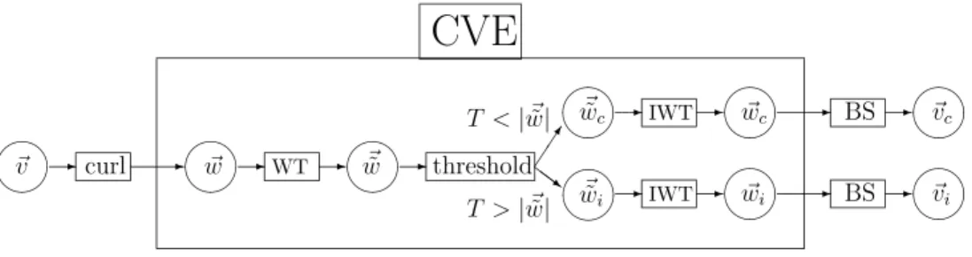
FIG. 1: Flowchart of the CVE decomposition.
III. COHERENT VORTEX EXTRACTION
The CVE decomposition uses an orthogonal three-dimensional multiresolution analysis (MRA) ofL2(IR3) ob-tained through the tensor product of three one-dimensional MRA’s ofL2(IR). In this context a function f ∈L2(IR3)can be developed into a three-dimensional wavelet basis
f(x) =
∑
γ∈Γ
fγψγ(x), γ= (j,ix,iy,iz,µ) (1)
wherejdenotes the scale,i= (ix,iy,iz)denotes the positions, µ=1, ...,7 indicates the 7 wavelets and the index setΓ={γ= (j,ix,iy,iz,µ) j=0, ...,J−1 ix,iy,iz=0, ...,2j−1 µ= 1, ...,7}. Due to orthogonality the wavelet coefficients are given by fγ=f ,ψγwhere·,·denotes theL2inner
prod-uct. For more details on this construction and on wavelets we refer the reader to the textbooks, e.g. [11] and also to the review article [1].
In the following applications, the Coifman 12 mother-wavelet is chosen. This mother-wavelet is almost symmetric and it has a compact support. Another point is that this wavelet has M=4 vanishing moments, and therefore the corresponding quadratic mirror filter has a length of 3M=12 [11].
We apply the extraction algorithm to a 3D vector valued vorticity fieldω=∇×v,wherev=v(x,y,z)is the velocity field. The three components ofωare developed into an or-thonormal wavelet series, from the largest scalelmax=20to the smallest scalelmin=2−J+1.
The vorticity field is decomposed into coherent vorticity ωc=ωc(x,y,z) and incoherent vorticityωi=ωi(x,y,z) by projecting its three components onto an orthonormal wavelet basis and applying nonlinear thresholding to the wavelet co-efficients. The choice of the threshold is based on theorems [7, 8] proving optimality of the wavelet representation for de-noising signals – optimality in the sense that wavelet-based estimators minimize the maximumL2-error for functions with
inhomogeneous regularity in the presence of Gaussian white noise. We have chosen the variance of the total vorticity in-stead of the variance of the noise, which gives the threshold T = (43ZlogN)12, whereZ =1
2ω,ωis the total enstrophy
(which is half the variance) andN3is the resolution. Notice that this threshold does not require any adjustable parameters. In summary, first we compute the modulus of the wavelet coefficients:
ω˜=
3
∑
n=1
˜ ωγ2n
1
2
. (2)
Then, the coherent vorticity is reconstructed from the wavelet coefficients whose modulus is larger than the thresh-oldT, while the incoherent vorticity is computed by the dif-ference with the total field. The two fields thus obtained,ωc andωi, are orthogonal, which ensures the decomposition of the total enstrophy intoZ=Zc+Zi.
The fast wavelet transform we use, requires a total number of operations of
O
(N), where N is the resolution.The CVE decomposition algorithm consists of three fast wavelet transforms (WT) for each vorticity component, a thresholding of the wavelet coefficients and three inverse fast wavelet transforms (IWT), one for each component ofω˜c, i.e., all coefficients with|ω˜|greater than the threshold, form the coherent vorticity (ωc). The incoherent vorticityωi com-ponents could be in principle computed using the inverse wavelet transform from the weak coefficients. In order to simplify computations we performed the difference between total and coherent vorticity which yields the same result. A flowchart of the CVE algorithm is depicted in Fig. 1. The induced coherent and incoherent velocity fields are computed using Biot–Savart’s law (BS),v=∇×(∇−2ω), from the
co-herent and incoco-herent vorticity fields, respectively using the fast Fourier transform. As we privilege a good compression rate rather than a perfectly denoised contribution we apply the algorithm using one iteration, that is to say, we apply the filtering with a threshold computed from the incoherent part [12].
IV. COMPARISON BETWEEN FILTERING VORTICITY
AND FILTERING VELOCITY
In the previous section we presented the classical CVE where we applied the wavelet filtering to the vorticity field and subsequently reconstructed the corresponding velocity fields. Here we apply the wavelet filtering to the velocity field to get the coherent and incoherent contributions and compare it to the filtering of vorticity. Then, we compute the corre-sponding coherent and incoherent vorticity fields. Due to the nonlinear thresholding employed in the wavelet filtering both procedures do not yield the same result. In Table I we can observe that the compression is slightly better in the modified CVE ,i.e., 1.68% instead of 3.59%. This happens because the velocity field is smoother than the vorticity field. On the other hand the vorticity field computed from the curl of this velocity field is less accurate than the one obtained using CVE filtering directly applied to the vorticity field.
CVE Filtering
based on vorticity based on velocity
total coherent incoherent total coherent incoherent
% of coeff. 100.00 3.59 96.41 100 1.68 98.32
Energy 2.96 2.95 0.01 2.96 2.94 0.02
% of Energy 100 99.70 0.30 100 99.50 0.50
Enstrophy 212.80 196.93 15.87 212.80 187.33 41.65
% of Enstrophy 100 92.54 7.46 100 88.03 19.57
TABLE I: Comparison of filtering CVE based on a decomposition of the flow field, corresponding to a Reynolds numberRλ=140, using Coifman 12 wavelets and Donoho’s thresholdT =1.52 for the velocity field andT=29.87 for the vorticity field.
the coherent part obtained with CVE approximates well the total vorticity. However, some peaks are over estimated. In the case when the modified CVE is used, the coherent part ap-proximates less well the total vorticity and the over estimation of the peak is worse.
(a) CVE 0 10 20 30 40 50 60 70 80
0 50 100 150 200 250
total coherent incoherent
(b) modified CVE
0 10 20 30 40 50 60 70 80
0 50 100 150 200 250
total coherent incoherent
FIG. 2: One dimensional cuts in thex-direction, fory=z=32∆x
with∆x= 2π
256for the modulus of vorticity|ω|for total field, coher-ent and incohercoher-ent fields atRλ=140.
This explains why slightly less energy (92.5%)is retained in the modified CVE compared to the energy retained using the vorticity based CVE (99.7%) as illustrated in Table I.
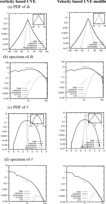
The PDFs and spectra of the velocity on vorticity fields that were obtained with the modified CVE filtering are shown in Fig. 3 (right). The velocity and vorticity PDFs and
spec-tra for the fields and the coherent contributions are similar to the ones presented in Fig. 3 (left) and that were obtained by the vorticity based CVE filtering. However the shapes of the PDFs of the incoherent fields differ for the two CVE methods. Indeed, in the case of the vorticity based CVE the PDFs of the incoherent velocity and vorticity fields are Gaussian and exponential decay, respectively, while in the case of the modi-fied velocity based CVE the PDFs are exponential for velocity and non exponential for vorticity. Moreover, the slopes of the spectra computed from incoherent part for both methods are different.
Vorticity based CVE Velocity based CVE modified
(a) PDF ofω
1e-07 1e-06 1e-05 0.0001 0.001 0.01 0.1 1
-150 -100 -50 0 50 100 150 total coherent incoherent Exponential fit
-30 0 30
1e-07 1e-06 1e-05 0.0001 0.001 0.01 0.1 1
-150 -100 -50 0 50 100 150 total coherent incoherent
-70 0 70
(b) spectrum ofω
1e-05 0.0001 0.001 0.01 0.1 1 10 100
1 10 100 total
coherent incoherent k^(1/3)
k^4 1e-05 0.0001 0.001 0.01 0.1 1 10 100
1 10 100 total
coherent incoherent k^(1/3) k^4
(c) PDF ofv
1e-07 1e-06 1e-05 0.0001 0.001 0.01 0.1 1 10
-8 -6 -4 -2 0 2 4 6 8 total coherent incoherent Gaussian fit
1
-0.4 0 0.4
1e-07 1e-06 1e-05 0.0001 0.001 0.01 0.1 1 10
-8 -6 -4 -2 0 2 4 6 8 total coherent incoherent Exponential fit
1
-1 0 1
(d) spectrum ofv
1e-05 0.0001 0.001 0.01 0.1 1 10
1 10 100 total coherent incoherent k^(-5/3) k^2 ( ) ( ) ( 1e-05 0.0001 0.001 0.01 0.1 1 10
1 10 100 total
coherent incoherent k^(-5/3) k^2
FIG. 3: PDF of the vorticity (a), velocity (c) (inset: PDF of the incoherent fields) and enstrophy (b) and energy (d) spectra for the total, coherent and incoherent fields, for the vorticity based CVE (left) and the modified velocity based CVE (right), forRλ=140.
In the following we discuss the results obtained with CVE based on the filtering of the vorticity fields and applied to the vorticity at resolutionN=2563andRλ=140.
part of the vorticity corresponds to 3.6% of the wavelet coefficients, which maintain 92.5% of the total enstrophy and 99.7% of the total energy.
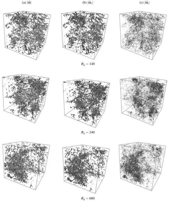
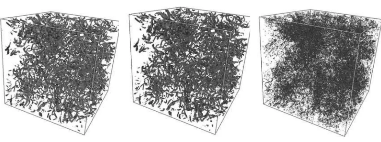
A visualization of the modulus of vorticity and their coher-ent and incohercoher-ent contributions are shown in Figure 4. We observe that almost all structures are preserved in the coher-ent part and there are no organized structures left in the inco-herent part. Indeed the total and coinco-herent part of the vorticity fields present vortex tubes and long filaments of vorticity. The incoherent part is noise-like.
In Figure 3 (left a), vorticity PDFs are plotted for the to-tal, coherent and incoherent parts. We find that the PDFs of the total and coherent fields almost coincide, exhibiting a stretched exponential behavior and a vorticity flatness about 8. The incoherent part shows a strongly reduced variance and the vorticity PDF has exponential tails (with flatness 4.92).
In Figure 3 (left b, d), the energy and the enstrophy spectra for the total, coherent and incoherent parts of the fields are illustrated. We observe that in the inertial range the coherent part presents similar energy and enstrophy spectra compared to the spectra of the total field, whereas they differ only in the dissipative range fork≥30.
V. RESULTS FOR OTHER REYNOLDS NUMBERS
In the following we study the influence of the Reynolds number. We apply the CVE to vorticity fields atRλ=240 and 680 computed at resolutionN=5123and 20483, respectively. For computational reasons, we only consider subcubes of size N=2563, and we apply the CVE to four subcubes to check if the statistics differ.
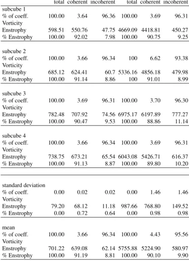
Table II summarizes the statistical properties of the vor-ticity for four different subcubes of size 2563extracted from theN=5123cube which correspond to a Reynolds number Rλ=240 and for four 2563subcubes of theN=20483 simu-lation which correspond to a Reynolds numberRλ=680.
ForRλ=240, the reconstruction of the coherent part of these fields requires only 3.6% of the wavelet coefficients and retains≈92% of the enstrophy, and forRλ=680 only ≈3.7% of the wavelet coefficients maintain about 91% of the enstrophy. Additionally, there are no significant changes in the skewness and flatness between the total field and the coherent field for the differentRλ. Moreover, we do not ob-serve significant variations between the statistical properties of the four different subcubes for eachRλ. The total, coher-ent and incohercoher-ent parts of the vorticity fields are visualized in Figure 4 forRλ=140,240 and 680. As observed in the Rλ=140 case, all structures are preserved in the coherent contribution and none remain in the incoherent contribution. However, with the increase ofRλ, we observe the presence of more structures in the analyzed subcubes.
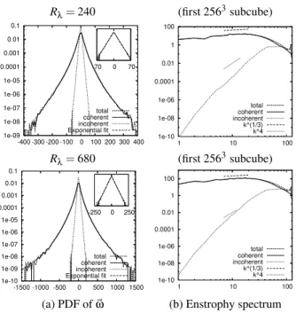
In Fig. 5 the PDFs of the vorticity and the enstrophy spec-tra for the total, coherent and incoherent fields are plotted for Rλ=240 and 680. They have the same behavior as the vor-ticity field forRλ=140, presented in Fig. 3 (a,b).
In [9] a related work was done also for homogeneous isotropic turbulence. The CVE was used for different resolu-tions 2563,5123,10243and 20483corresponding toRλ=167, 257, 471 and 732, respectively. The main difference is that
Rλ=240 Rλ=680
total coherent incoherent total coherent incoherent
subcube 1
% of coeff. 100.00 3.64 96.36 100.00 3.69 96.31
Vorticity
Enstrophy 598.51 550.76 47.75 4669.09 4418.81 450.27
% Enstrophy 100.00 92.02 7.98 100.00 90.75 9.25
subcube 2
% of coeff. 100.00 3.66 96.34 100 6.62 93.38
Vorticity
Enstrophy 685.12 624.41 60.7 5336.16 4856.18 479.98
% Enstrophy 100.00 91.14 8.86 100 91.01 8.99
subcube 3
% of coeff. 100.00 3.69 96.31 100.00 3.70 96.30
Vorticity
Enstrophy 782.48 707.92 74.56 6975.17 6197.89 777.27
% Enstrophy 100.00 90.47 9.53 100.00 88.86 11.14
subcube 4
% of coeff. 100.00 3.66 96.34 100.00 3.69 96.31
Vorticity
Enstrophy 738.75 673.21 65.54 6043.08 5426.71 616.37
% Enstrophy 100.00 91.13 8.87 100.00 89.80 10.20
standard deviation
% of coeff. 0.00 0.02 0.02 0.00 1.46 1.46
Vorticity
Enstrophy 79.20 68.12 11.18 987.66 768.80 149.52
% Enstrophy 0.00 0.72 0.64 0.00 0.98 0.98
mean
% of coeff. 100.00 3.66 96.34 100.00 4.43 95.56
Vorticity
Enstrophy 701.22 639.08 62.14 5755.88 5224.90 580.97
% Enstrophy 100.00 91.19 8.81 100.00 90.10 9.90
TABLE II: Statistical properties of the vorticity field for the 2563 subcubes extracted from the 5123and 20483 which correspond to Reynolds numbersRλ=240 andRλ=640, respectively. The value of Donoho’s threshold used for the subcubes 1 to 4 forRλ=140 are
51.18, 56.39, 61.55 and 58.56, respectively. The value of Donoho’s threshold used for the subcubes 1 to 4 forRλ=640 are 152.23, 157.58, 192.21 and 174.20, respectively.
(a)|ω| (b)|ωc| (c)|ωi|
Rλ=140
Rλ=240
Rλ=680
FIG. 4: Modulus of vorticity for total (a), coherent (b), and incoherent (c) parts.Rλ=240 andRλ=680 subcubes 2563are visualized to zoom on the structures. The values of the isosurfaces areσ140=56,σ240=96 andσ680=290 for total and coherent parts andσ140=14,σ240=24 andσ680=75.2 for the incoherent part.
VI. GEOMETRICAL STATISTICS
VI.1. Helicity
To get insight into the geometrical statistics of the flow we study the helicity [13] defined by
H(v,ω) =v·ω.
To study the effect of CVE we split the helicity into four contributions, namely
Hcc=h(ωc,vc), Hic=h(ωi,vc), Hci=h(ωc,vi), Hii=h(ωi,vi),
corresponding to the coherent and incoherent contributions of the velocity and vorticity components.
max-Rλ=240 (first 2563subcube) 1e-09 1e-08 1e-07 1e-06 1e-05 0.0001 0.001 0.01 0.1
-400 -300 -200 -100 0 100 200 300 400 total coherent incoherent Exponential fit
-70 0 70
1e-10 1e-08 1e-06 0.0001 0.01 1 100
1 10 100
total coherent incoherent k^(1/3) k^4
Rλ=680 (first 2563subcube)
1e-10 1e-09 1e-08 1e-07 1e-06 1e-05 0.0001 0.001 0.01 0.1
-1500 -1000 -500 0 500 1000 1500 total coherent incoherent Exponential fit
-250 0 250
1e-10 1e-08 1e-06 0.0001 0.01 1 100
1 10 100
total coherent incoherent k^(1/3) k^4
(a) PDF ofω (b) Enstrophy spectrum
FIG. 5: PDF (left) of vorticity (inset: PDF of the incoherent fields) and enstrophy spectrum (right) for the total field, coherent and inco-herent parts.
imize the relative helicity, defined as
h(v,ω) = v·ω ||v|| ||ω||.
Such a characterization corresponds to a special case of nonlinearity depletion. However the latter does not prove that we have extracted all coherent vortices using the CVE decom-position. Also the relative helicity is split into four contribu-tions, namely
hcc=h(ωc,vc), hic=h(ωi,vc), hci=h(ωc,vi), hii=h(ωi,vi).
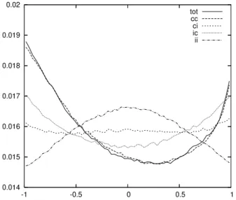
In Fig. 6 we show visualizations of the relative helicity for the four components. Almost all of the structures are present in thehcccomponent. We can observe also some small struc-tures inhci andhic, and no more structures inhii. This can also be observed in the PDF of the helicity. The PDFs of the different contributions of relative helicity are plotted in Fig-ure 7. The coherent velocity,i.e.eitherhccorhic, exhibits the same PDF as the one of the total flow, with two maxima at h=±1 for the relative helicity.
This corresponds to helical vortex tubes for which velocity and vorticity vectors are either parallel or anti–parallel, re-spectively. On the other hand, the PDF of the relative helicity based on the incoherent velocity and the incoherent vortic-ity,i.e.,hii, is maximal ath=0 which suggests a tendency towards two-dimensionalization.
VI.2. Theλ2criterion
The coherent nature of the structures extracted by wavelet analysis can be assessed by comparing the coherent structures
educed from both the total and wavelet-filtered flow fields by means of one of the classical criteria used to define a vortex core. Among these criteria, theλ2[14] criterion is of interest
since it yields an accurate eduction of the vortices, whereas the physical analysis on which it is based is not directly re-lated to the vorticity. It therefore allows a fair analysis for the accuracy of the vorticity-based wavelet extraction.
The key idea behind the λ2 criterion is to seek for
re-gions exhibiting relative minima of pressure classically as-sociated with vortical structures while discarding viscous and unsteady effects that are not related to the vortex physics. Af-ter some rearrangements of the incompressible Navier-Stokes equations taking into account these restrictions (see Jeong and Hussain[14] for details), the Hessian tensor of pressure
H
(p)is approximated by the opposite of the tensor S2+Ω2where S andΩ, respectively, stand for the symmetric and anti-symmetric part of the velocity gradient tensor. Regions of pressure minima are characterized by two positive eigenval-ues for the pressure Hessian, implying that the second high-est eigenvaluesλ2of the tensor S2+Ω2is negative in such
regions. Vortex core in the sense of theλ2criterion are
con-sequently educed by the condition :
λS2+Ω2
2 <0
The original definition of theλ2criterion is generally
use-less for visualization of fully turbulent flows since it yields the eduction of a very large amount of the total volume. One way to alleviate this drawback is to arbitrary set a threshold lower than the original 0-valued one. From a mathematical view-point, it implies that only the vortex core exhibiting the steep-est pressure minima are highlighted. Physically, the cores thus educed correspond to the strongest and most coherent structures.
The value of the isosurface has been set for the present analysis to a value roughly equal to the twice of the oppo-site of the standard deviation ofλ2over the whole
computa-tional volume. It is worth noting that the values of the stan-dard deviation found for the total and coherent flow field are almost identical. Consequently, the same eduction threshold has been applied to both flow fields. Structures educed from the total and coherent flow field are displayed in Figs. (8) (a) and (b), which demonstrate that the original topology of the vortices is almost perfectly recovered from the coherent part of the wavelet-filtered flow field. On the contrary, if the value of the isosurface level is increased up to four times the op-posite of theλ2standard deviation value over the incoherent
flow field, as seen in Fig. 8 (c), structures are indeed educed but they are of small sizes, being almost isotropic in shape, and they hardly exhibit any spatial organization. It can there-fore be concluded that the λ2 analysisa posteriori
demon-strates that the CVE effectively result in the extraction of co-herent vortices in one of the most widely accepted sense.
VII. FINAL REMARKS
(a)|h| (b)|hcc|
(c)|hci| (d)|hic| (e)|hii|
FIG. 6: Total helicity (a) and the four contributions of relative helicity forRλ=140. The isosurfaces are|σ|=|σcc|=0.97 (b),|σci|=0.95
(c),|σic|=0.95 (d) and|σii|=0.94 (e). The red color indicates positive isosurfaces and the blue color negative values.
0.014 0.015 0.016 0.017 0.018 0.019 0.02
-1 -0.5 0 0.5 1
tot cc ci ic ii
FIG. 7: PDFs of the relative helicity for the total and the four contri-butions.
random background flow, which is structureless and decorre-lated. The above results hold for all Reynolds numbers we investigated. So we have shown that the CVE method is an efficient tool for extracting coherent vortices out of turbulent flows.
From the present results we conjecture that modeling the
effect of the discarded modes on the resolved modes is eas-ier to perform using the Coherent Vortex Simulation (CVS) approach introduced in [4, 15]. CVS computes all degrees of freedom which contribute to the flow nonlinearity,i.e., the coherent modes, whatever their scale, while the remaining de-grees of freedom,i.e., the incoherent modes, are discarded to model turbulent dissipation. The method actually combines an Eulerian projection of the solution with a Lagrangian pro-cedure for the adaption of the computational basis: for more details we refer the reader to [15]. The next step to demon-strate the potential of CVS is to develop an adaptive wavelet solver for the 3D Navier–Stokes equations.
Acknowledgments
Cen-(a)λ (b)λc (c)λi
FIG. 8: Coherent structures educed by theλ2criterion from the total flow field (a), the coherent flow field (b), and the incoherent flow field (c). The isosurfaces visualized areσ=0.2 (a),σc=0.2 (b), andσi=0.02 (c).
trale Marseille.
Related papers can be downloaded from the following
web-page: ’http://wavelets.ens.fr/’
corresponding author: [email protected]
[1] M. Farge, Annu. Rev. of Fluid Mech.24, 395 (1992).
[2] M. . Domingues, I. Broemstrup, K. Schneider, M. Farge, and B. Kadoch, ESAIM: Proc.16, 164 (2007).
[3] M. Farge, G. Pellegrino, and K. Schneider, Phys. Rev. Lett.87, 054501 (2001).
[4] M. Farge, K. Schneider, and N. Kevlahan, Phys. Fluids11, 2187 (1999).
[5] M. Farge, K. Schneider, G. Pellegrino, A. A. Wray, and R. S. Rogallo, Phys. Fluids15, 2886 (2003).
[6] K. Schneider, M. Farge, G. Pellegrino, and M. Rogers, J. Fluid Mech.534, 39 (2005).
[7] D. Donoho, Appl. Comput. Harmon. Anal.1, 100 (1993). [8] D. Donoho and I. Johnstone, Biometrika81, 425 (1994). [9] N. Okamoto, K. Yoshimatsu, K. Schneider, M. Farge, and
Y. Kaneda, Phys. Fluids19, 115109 (2007).
[10] P. Yeung, D. Donzis, and K. Sreenivasan, Phys. Fluids 17, 081703 (2005).
[11] I. Daubechies,Ten Lectures on wavelets, vol. 61 (CBMS-NSF Conferences in Applied Mathematics, SIAM, 1992).
[12] A. Azzalini, M. Farge, and K. Schneider, Appl. Comput. Har-mon. Anal.18, 177 (2005).
[13] H. K. Moffatt, J. Fluid Mech.150, 359 (1985). [14] J. Jeong and F. Hussain, J. Fluid Mech.285, 69 (1995). [15] M. Farge and K. Schneider, Flow Turbul. Combust.66, 393
(2001).
[16] J. Clyne, P. Mininni, A. Norton, and M. Rast, New J. Phys.9, 301 (2007).