Reaction-Diffusion Stochastic Lattice Model for a Predator-Prey System
´Attila L. Rodrigues and Tˆania Tom´e Instituto de F´ısica
Universidade de S˜ao Paulo Caixa postal 66318 05315-970 S˜ao Paulo- SP, Brazil
Received on, 17 December, 2007
We have the purpose of analyzing the effect of explicit diffusion processes in a predator-prey stochastic lattice model. More precisely we wish to investigate the possible effects due to diffusion upon the thresholds of coexistence of species, i. e., the possible changes in the transition between the active state and the absorbing state devoid of predators. To accomplish this task we have performed time dependent simulations and dynamic mean-field approximations. Our results indicate that the diffusive process can enhance the species coexistence.
Keywords: Stochastic models; Predator-prey systems; Reaction-diffusion systems; Mean-field approach; Numerical simula-tion
I. INTRODUCTION
Computational physics descriptions and the usual analysis of numerical simulation data provided by the statistical me-chanics can give worthy contributions to the study of pop-ulation biology problems. A basic, but not trivial, issue of population biology, is the one concerned to the dynamics of a predator-prey system. This problem has been considered from the theoretical point of view since Lotka who in 1920 [1], [2], [3], followed by Volterra [4], has introduced the first model (to be called here LV model) able to elucidate the main features of species interactions and populational cycles in predator-prey systems. After that, the LV model has been modified to contemplate other important features of these systems and we may say that most of the theoretical approaches presently used to describe problems of the population biology have some ba-sis on the LV model. Among those descriptions we point out the stochastic lattice gas models approach [5], [6], which will concern us in the present article. These models are able to provide spatial patterns of species distribution which can be coupled to local time oscillations as well as other important features of predator-prey systems [7], [8], [9], [10].
Doubtlessly a mark in the understanding of predator-prey interactions, and their coexistence in space distributed sys-tems, is the experiment on predation performed by Huffaker in 1958 [11]. He has verified that an heterogeneous habitat can be crucial to maintain the coexistence of species for a long pe-riod of time. Experiments performed in homogeneous habitat have shown that predators eat prey very quickly, prey get ex-tinct and then predators die of starvation. These experimental results have evidenced that the coexistence of species for a long period of time can be directly related to a heterogeneous spatial distribution of the individuals of each species. Partic-ularly, this feature should be taken into account in the mod-elling of predator-prey systems which population sizes can at-tain very small values, or when populations loose contact and become isolated during some period of time. That is, when the species populations are spatially distributed.
Much of the theoretical developments to describe the rˆole of space in population biology problems were, in a certain way,
motivated by the Huffaker’s experiments. We detach two rel-evant stochastic approaches which take into account the local-ization of species individuals and their local interactions: (i) the stochastic lattice gas models, also calledinteracting par-ticle systems[7], [8]; (ii) the metapopulation approaches and patch models[12], [13], [14], [15]. In the last decades, both approaches have been largely used to analyze, at different lev-els of description, the different features of population biology problems. Several investigations have been developed in this issue and here we just cite some of them [7]-[10], [12]-[41].
In the present article we are concerned on the effect of dif-fusive processes in predator-prey systems described by the stochastic lattice model introduced by Satulovsky and Tom´e [9]. However, before entering into the details of our stochas-tic dynamic analysis, we will briefly expose, in what follows, the main features of the LV model, as well as related models; patch models and spatial models for predator-prey systems are also exposed. This is not a review on theoretical approaches of population biology, but a very basic, brief and simple expla-nation ofsomeof the features ofsometheoretical approaches. Our purpose is just to clarify the issue treated in the present article.
A. Lotka-Volterra model and related models
The definition and description of the dynamics of predator-prey system consists in one of the fundamental problems of the population biology. One considers two species, predator and prey, sharing the same habitat. To understand the dynam-ics of coexistence of both populations it is necessary to estab-lish the main characteristics of their interaction. We depart from the LV model for a predator-prey system which is de-fined by a set of two ordinary differential equations for prey size population, denoted byH, and predators size population, denoted byP. This description is based on the law of mass action and the differential equations can be written in the fol-lowing form
dH
dP
dt =r2H P−r3P, (2)
wherer1,r2 andr3 are nonnegative constants related to the processes considered in the LV model. The process of prolif-eration of prey is proportional to the prey number, which is expressed by the term(r1H)in Eq. (1). Thus, in the absence of predators the prey population size increases exponentially in time. This result comes from the assumption that there is an unlimited amount of resources and space for prey prolifera-tion. The predator-prey interaction, the most relevant and cru-cial process, is expressed as the product of predators number and the prey number (term(r2HP)in Eqs. (1) and (2)). Ac-cording to this autocatalytic process, predators increase their number just when consuming prey and there is just one prey species available for them. Finally, predators size population decreases according to a spontaneous process which occur at rater3. It is worth to note that it is implicitly assumed in the LV model that predators and prey populations are very well mixed in an homogeneous habitat. These are usual presup-poses when one uses the law of mass action, as it was used to derive all terms of Eqs. (1) and (2). In this case the predator-prey system can be described at any instant of timetonly by their size populations, that is, by(H(t),P(t)).
The trivial solution of Eqs. (1) and (2) is unstable and the non-trivial one is a center for which any perturbation around is periodic. Once an initial condition is fixed we can say that both population sizes oscillate in time with the same period, out-of-phase and a peak in the prey number is always followed by a peak in the predators number. These are relevant features of the population cycles encountered in experiments on pre-dation [11] and in nature. In this case, a famous example con-sists on the long term data related to the population cycles of the snowshoe hare and the lynx of the Canadian boreal forest [43], [44], [45], [46], [47], [48], [49].
However, the LV model displays infinitely many periodic orbits in theP−Hphase plane and these are related to differ-ent initial conditions [44]. In this respect the LV model fails in describing biologic populations, since it is not expected that a small change on the initial assumptions will lead to differ-ent population cycles [48]. In order to answer for the stabil-ity of a predator-prey system important modifications in the LV model were performed. One of them consists in taking into account the fact that there exists a maximum prey pop-ulation size that the system can support since the amount of food for prey proliferation is not unlimited. This feature can be expressed by the consideration of a logistic term to describe prey proliferation. So that the first term in Eq. (1) is replaced byr1H(1−H/C), whereCis a constant related to the maxi-mum prey number, and the constantr1is the prey reproduction rate (in the absence of predators). The resulting modified LV model predicts stable nontrivial solutions which are attained by damped oscillations of the population sizes. Another rel-evant modification of the LV model that has been considered concerns to the response of predators to prey population size changes, the so called functional responses f(H)[48]. One consider the term related to predator-prey interaction in Eqs. (1) and (2) written as(r2 f(H)P). In the original LV model f(H)is linear; in general it is stated according to the
biolog-ical effect to be described. Interesting functional responses where considered by Holling and Tanner [47]. Their models, forspecific sets of parameters, are able to predict species co-existence which can be stable or related to population cycles. These sets of parameters and the different models seem to de-scribe qualitatively some predator-prey systems observed in nature [50].
B. Patch models
A more sophisticated approach to describe the dynamics of a predator-prey system can be attained considering patch models and the metapopulation models approaches [13], [14]. This description was primordially considered by Levins in 1969 [42] to analyze a single species system whose individu-als can proliferate and die at given rates. The main feature captured in the Levins approach relies in the fact that it is capable to recognize the necessity of taking into account the space available for the species proliferation. In the metapopu-lation approach it is considered that the popumetapopu-lation can be sub-divided in subpopulations which live in interconnected habitat patches. Instead of treating the dynamics of the entire popu-lation sizes, one treats the dynamics of the fraction of patches occupied by species individuals. The most simple patch for-mulation, as stated by Levins, consists of an ordinary differ-ential equation for the fraction of patches occupied by the species individuals; this equations is build up on the basis of the law of mass action. A natural extension of Levins ap-proach for a two-species system, as a predator-prey system, could be accomplished considering three types of patches: empty patches, patches occupied by prey and patches occu-pied by predators. The dynamics of such a model can be stated as follows: prey can proliferate in empty patches with a given ratea, predators can proliferate in prey patches at rate b, and can die, leaving an empty patch, with a given ratec. In this context a simple description, which takes into account the LV model mechanism of interaction between the two species, may be given by,
dx
dt =ax(1−x−y)−bxy (3)
dy
dt =bxy−cy, (4)
set of Eqs. (3) and (4) differ from the structure of the set of Eqs. (1) and (2) just by the logistic term. This patch model display nontrivial stable stationary solutions corresponding to stable coexistence of prey and predators.
The metapopulation approach has been developed to in-clude local stochastic dynamics and is nowadays largely used to model ecological problems. One of the issues investigated in the scope of this approach concerns to the dynamics of species distributed over fragmented habitats. A relevant prob-lem treated in this case concerns the relationship between the fragmentation of the habitat and the conservation of species and biodiversity [14], [29], [37].
C. Stochastic lattice models
Theoretical descriptions based on the assumptions of the LV modified models, as the ones above described, can be ad-equate if we want to describe the dynamics of species popu-lations which are mixed and dispersed over an homogeneous space. In this case the descriptive level of the population dy-namic problem is such that the spatial structure is not relevant. However, under certain circumstances, one needs a theoretical approach which takes into account the spatial structure of the habitat and the localization of the individuals of each species. So, we need to establish the level of description needed and desired to describe a given population biology problem. This problem has been very well placed by Durrett and Levin [7]. They have treated the dynamics of a biological population problem by considering different levels of description and, consequently, different theoretical approaches.
That study gives particular attention to the approach based on stochastic lattice gas models, also called interacting par-ticle systems [5, 6], which has been largely exploited, in the last years. A multiplicity of works have evidenced the im-portance of spatial structured models to describe ecological problems [7], [8]. The approach of the stochastic lattice gas models is based on Markovian processes defined on discrete spaces, which are able to take into account the localization of discrete individuals of a given population. Such a description allows us to treat the important features for the determination of the thresholds of species coexistence, and spatial patterns of distribution of the species individuals, by considering simple models [10], [27], [32]. Usually the spatial stochastic struc-tured models are studied by means of computational simula-tions and dynamic mean-field approximasimula-tions.
One of the first systematic statistical mechanics analysis of a very simple stochastic lattice model for a predator-prey sys-tem was performed by Satulovsky and Tom´e in 1994 [9]. The model, to be calledST model, is able to exhibit local time os-cillations of species populations and stable coexistence. Other deeper investigations on this model and similar models fol-lowed [10], [27], [28], [34], [38]. The ST model has a phase diagram displaying an active phase, where there is species coexistence with local time oscillations and coexistence with stationary densities; it also exhibits an absorbing phase which correspond to the extinction of one of the species. A version
of the ST model with synchronous updating, a PCA, was con-sidered by de Carvalho, Tom´e and Arashiro [10, 31, 33, 38]. In this case it has been shown [38] that the whole transition line between the active and absorbing states is a line of criti-cal points which belongs in the directed percolation universal-ity class but one point belonging in the dynamic percolation universality class [16].
It is worth to note that mean-field approaches for spatial models, as the ST model [9] and its synchronous version [40] are able to provide species coexistence with self-sustained coupled time oscillations which are attained from a regime of stable coexistence by a Hopf bifurcation. The oscillations are stable against any perturbation on the initial conditions and they have a very well defined amplitude and period. The lat-ter is the same for the prey density time series and predators density time series, and an abundance of prey is always fol-lowed by an abundance of predators. However, if the spatial structure of these models is explicitly considered, for exam-ple, when one performs Monte Carlo simulations on square lattices, it can be verified that the amplitude of oscillations decays as the system size increases; and, it vanishes in the thermodynamic limit [9], [33]. Therefore, oscillations are not globally synchronized, but remain synchronized in finite and small regions of the space; these are called local oscillations and have the property of being coupled to heterogeneous and interesting spatial patterns of species distribution.
The same behavior is observed for other spatial models [8]: coexistence with time oscillations resulting from Hopf bifur-cations provided by mean-field approaches, and local oscil-lations with pattern formation when the spatial structure of the model is indeed considered. From these results we could infer that population cycles observed in nature and in experi-ments may be synchronized at subregions of the habitat. How-ever, we must be careful with these results, since, usually, the predator-prey lattice models are still to crude to be directly compared with data obtained from experiments and from col-lected data for population cycles in nature. We can drawn some analogies and try to capture the fundamental proper-ties of prey-predator systems. For example, the ST model [9], exhibits for a given range of the model parameters, pro-nounceable predator and prey oscillations [10] which seem to be qualitatively similar to the hare-linx population cycles. However, until now, it was not included in this model the in-herent features, as intrinsic population growth rates, which al-lows us to make direct relationships between the theoretical description and the observed population cycles.
D. Scope of this article
an absorbing state. We also perform mean-field approxima-tions. In section II we define the predator-prey stochastic model with diffusion. In section III we analyze the model by means of simple and pair mean-field approximations. In section IV we show our computational simulation results and in section V we present a discussion of our results.
II. PREDATOR-PREY STOCHASTIC LATTICE MODEL
WITH DIFFUSION
We model a predator-prey system by a Markovian stochas-tic dynamics defined in a discrete space where individuals of each species are localized. The dynamics is asynchronous and comprehends a set of subprocesses which mimic the re-action processes of birth, death and predation and the explicit movement of individuals of each species by diffusive local processes.
We consider a regular lattice which represents the habitat where individuals can survive and interact with each other. For each site i on the lattice, i=1,2, ...,N, we associate a stochastic discrete variable ηi which can take the values: 1, if siteiis occupied by a prey individual; 2, if siteiis occu-pied by a predator and 0, if siteiis empty. Each site can be occupied by at most one individual. The stochastic dynam-ics is defined over the configurational space spanned by the stochastic vector,η= (η1,η2, . . . ,ηN), the microscopic state. The time evolution of the probabilityP(η,t)associated to the stochastic vectorηat timetis given by the master equation,
d
dP(η,t) =
∑
η′W(η|η′)P(η′,t)−W(η|η′)P(η′,t)
, (5)
whereW(η|η′) =w(η|η′)/τis the conditional transition rate, fromη′= (η′
1,η′2, . . . ,ηN′ )toη, andw(η|η′)is defined by the expression,
w(η|η′) =d wdiff(η|η′) + (1−d)wreact(η|η′), (6) wheredis the probability of diffusion,wdiff(η|η′)denotes the conditional probability transition associated to the diffusive processes andwreact(η|η′)denotes the conditional probability transition associated to the reactive processes. In what follows we define each of these processes.
i)Diffusion. The possible diffusion processes are: X+Z⇄Z+X,
Y+Z⇄Z+Y,
X+Y⇄Y+X,
whereX denotes prey (ηi=1),Y denotes predators (ηi=2) andZ denotes a vacant site (ηi=0), that is, food supply for prey and therefore a source for prey proliferation. We chose at random a pair of nearest neighbors sitesiand j. After that we exchange the states of these two sites with probabilityd. We define the transition probability associated to this process,
which was denoted in expression (6) by wdiff(η|η′), as
fol-lows:
wdiff(10|01) =δ(ηi,1)δ(ηj,0) +δ(ηi,0)δ(ηj,1), (7) which is related to diffusion of prey in empty sites;
wdiff(12|21) =δ(ηi,1)δ(ηj,2) +δ(ηi,2)δ(ηj,1), (8) which is related to diffusion of prey between prey and preda-tors;
wdiff(20|02) =δ(ηi,2)δ(ηj,0) +δ(ηi,0)δ(ηj,2), (9) which is related to diffusion of predators in empty sites.
ii)Reactions. The possible reaction processes are X+Z→X+X
X+Y →Y+Y
Y→Z and the cyclic process
X→Y→Z→X for the local reactions are always observed.
At each time step we choose a sitei at random and it is updated according to the following set of local rules:
(a)Prey birth. If siteiis empty then it can be occupied by a prey and the transition probability per site associated is
wreact(1|0) =aδ(ηi,0) 1
z
∑
j δ(ηj,1), (10) where the summation is over the nearest neighbor of sitei,ais a parameter related to the prey birth probability,zis the coor-dination number of lattice,δ(x,y)denotes here the Kronecker delta.(b)Predation and predators birth. The process of predation is accompanied by the instantaneous death of prey and birth of predator. If the siteiis occupied by prey then in the next instant of time, with probability
wreact(2|1) =bδ(ηi,1) 1
z
∑
j δ(ηj,2), (11) wherebis a parameter related to the predation probability, site iwill be occupied by a predator;(c)Death of predators. The third reactive process is related to the death of predators, which happens spontaneously, with probability
0 0.2 0.4 0.6 0.8 1
d
0.15 0.2 0.25 0.3
c
FIG. 1: Phase diagram in the planecversusd, obtained from pair mean-field (upper curve) approximation and from numerical simula-tions (lower curve), wherecis the predator death probability andd is the diffusion probability. The probabilityaof prey birth and the probabilitybof predation are equal,a=b=1−c. The full circle corresponds to the transition point given by the simple mean-field approximation.
III. DYNAMIC MEAN-FIELD APPROXIMATION
We analyze the model by means of two levels of mean-field approximation: the simple (SMF) and pair (PMF) approxima-tion [39, 52]. In the SMF, the probability of a cluster of sites is approximated by a product of one-site probabilities. In this case it suffices to consider the time evolution for the density of preyx=P(1)and the density of predatory=P(2). The time evolution equations, obtained from the master equation, assuming that space is homogeneous and isotropic, are given by
dx
dt =ax(1−x−y)−bxy (13) and
dy
dt =bxy−cy (14)
The solution of these equations gives a continuous phase tran-sition from an active state (0≤x≤1, 0≤y≤1) to a prey absorbing state (x=1, y=0) occurring at b=c. Here we are considering only the case a=b which implies that the transition occurs at cSMFcrit =1/3 [9, 25]. We point out that this approximation is not able to take into account explicitly the diffusion process so the resulting transition line does not depend ond. We note that equations (13) and (14) have the same form of equations (3) and (4) which were devised under the assumptions of a patch model.
PMF is the first approximation that is able to shown prop-erties that depends explicitly on the diffusion. In this approxi-mation correlations of higher order are written in terms of one-site and two-one-site probabilities. Assuming again that space is homogeneous and isotropic it suffices to use the two densities
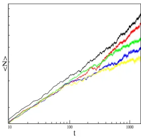
10 100 1000
t
<N>
FIG. 2: Log-log plot of the time evolution of the mean number of predatorsN. The figure shows the behavior of this quantity for a=b,d=0.2 and for five values ofc: 0.2348, 0.2350, 0.2354, 0.2356 and 0.2358, from top to bottom.
x=P(1)andy=P(2)and three nearest neighbor pair corre-lationsu=P(10),v=P(12)andw=P(20). The time evo-lution equations for these variables are too cumbersome and will not be written down. These equations are integrated nu-merically by repeated iterations to get the stationary solutions. Figure 1 shows the transition line in the spacecversusd for the casea=b. We see that as one increases the value of dif-fusion probabilityd the transition from the active (where the species coexistence takes place) to the absorbing state occurs at higher values ofc. That is, the diffusion process enhances the coexistence of species. We see that the transition line ap-proaches the simple mean-field value,c=1/3, for sufficiently large diffusion,d=1.
IV. SIMULATIONAL RESULTS
The simulation procedure is carried out as follows. At each time step we choose a random numberζhomogeneously dis-tributed between 0 and 1. Ifζ<d, the diffusion process is carried out. Otherwise the reactions of birth, death and preda-tion are realized. That is, the diffusion , described by Eqs. (7), (8) and (9), occur with probability d and the reaction processes (10), (11) and (12) occur with probabilities(1−d)a, (1−d)band 1−d)c, respectively. We are also assuming that a+b+c=1.
100 1000
t
0,1
P
FIG. 3: Log-log plot of the time evolution of the survival probability P. The figure shows the behavior of this quantity fora=b, d=
0.2 and for five values ofc: 0.2348,0.2350, 0.2354, 0.2356 and 0.2358, from top to bottom.
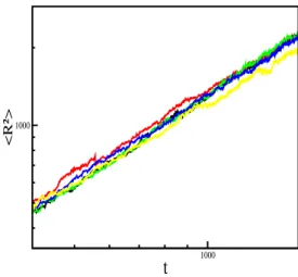
number of predatorsN, the survival probabilityP, i.e. the probability of having at least one predator in the lattice at time t. We also have analyzed the mean-square distance of spread-ing of activity from the origin, R2, as a function of time. Each run is initiated by randomly chosen one site and them the rules defined in Eqs. (6)-(12) are applied. The updating is asynchronous and we consider lattice sizes sufficiently large so that predators do not reach the borders of the lattice during the simulation time.
According to the scaling laws for time dependent simula-tions [51] at criticality the following asymptotic behaviors are expected,
N ∼ tη, P∼ t−δ, R2 ∼ tz, (15) whereη,δandzare dynamic critical exponents.
Figures 2, 3 and 4 show the behavior ofN,P(t)andR2 as a function of time for a given set of parameters a, band d=0.2 and different values ofcnear criticality. According to the scaling relations (15) a straight line fitted to the data points in the log-log plot of these quantities allow us to obtain the lo-calization of the critical point. Using the parametrization in-troduced in [9], [10], we can express the parametersa,bandc,
asa= (1−c)/2−p,b= (1−c)/2+p, with−1/2≤p≤1/2 and 0≤c≤1−2|p|. Forp=0.0 we estimate that the transi-tion from the active state to the absorbing state, and diffusion probabilityd =0.2, occurs at c1crit =0.2354. For the same set of parameters, but without explicit diffusion (parameter d=0.0), it has been obtainedc0
crit=0.1816(1)[9].
The exponent values were determined performing 100 sim-ulations, each one with 5000 independent runs. Each simula-tion contributes with a value of the exponents in a histogram. The exponent values are estimated as the mean value of the associated distribution and the statistical errors are achieved
1000
t
1000
<R²>
FIG. 4: Log-log plot of the time evolution of the mean square dis-tance of spreading of predatorsR2. The figure shows the behav-ior of this quantity for a=b, d=0.2 and for five values of c: 0.2348,0.2350, 0.2354, 0.2356 and 0.2358, from top to bottom.
through the standard deviations. As long as the histogram dis-tribution is compatible with a Gaussian disdis-tribution, the use of this method can provide lower statistical errors with more simulations. If the histograms become incompatible with a Gaussian distribution then the errors can not be evaluated in such a way. In this case, the relevant error is the one associated to the critical value ofc.
Considering this procedure we get the following esti-mates for the values of the dynamic critical exponents: η= 0.236(5),δ=0.441(8)andz=1.129(8). Then, within the statistical errors, the values for the exponentsη,δandz, seem to be in agreement with the ones of the directed percolation universality class [5].
Finally, we observe that our numerical results show that, for the set of parameters considered here, the threshold of coexis-tence of species increases when the explicit diffusion process is considered.
V. DISCUSSION
transi-tion from the active state (coexistence of species) to the prey absorbing state. The phase transition is continuous and seem to belong to the directed percolation universality class as it occurs for null diffusion.
It is worth noticing that the enlargement of the active phase is a consequence of the type of diffusive processes we have considered. The fact that prey can move over the lattice pro-motes their birth in empty sites and the meeting with preda-tors. This gives place to the possible predation and birth of predators. Then the number of predators is increased even when their probability of deathcis considerably high. The movement of prey promotes the mixing of the space. For high values of diffusion the critical line given by the pair mean-field approximation approaches very quickly the simple mean-field
result where the transition from the active state to the prey absorbing state occurs atcSMF
crit =1/3 fora=b(the set of pa-rameters considered here).
In future work we plan to obtain the whole phase diagram of the model, as well as to analyze the possible types of species coexistence, for different values of the diffusion probability by means of extensive numerical simulations.
Acknowledgment
T. T. is obliged to J. A. Plascak, chairman of the V Brazil-ian Meeting on Simulational Physics, for the meeting invita-tion. The authors have been supported by the Brazilian agency CNPq.
[1] A. Lotka, J. Am. Chem. Soc.42, 1595 (1920).
[2] A. Lotka,, Proc. Nat. Acad. of Sciences USA 6, 410 (1920). [3] A. Lotka, Elements of Mathematical Biology (Dover, New
York, 1924).
[4] V. Volterra, Lec¸ons sur la Th´eorie de la Lutte pour la Vie (Ghautier-Villars, Paris, 1931).
[5] J. Marro and R. Dickman,Nonequilibrium Phase Transitions in Lattice Models (Cambridge University Press, Cambridge, 1999).
[6] T. Tom´e e M. J. de Oliveira, Dinˆamica Estoc´astica e Ir-reversibilidade(Editora da Universidade de S˜ao Paulo, S˜ao Paulo, 2001).
[7] R. Durrett and S. Levin, Theor. Popul. Biol.46, 363 (1994). [8] R. Durrett and S. Levin, J. Theor. Biol.205, 201 (2000). [9] J. E. Satulovsky and T. Tom´e, Phys. Rev. E49, 5073 (1994). [10] K. C. de Carvalho and T. Tom´e, Int. J. Mod. Phys. C17, 1647
(2006).
[11] C. B. Huffaker, Hilgardia27, 343 (1958). [12] S. A. Levin, Am. Naturalist108, 207 (1974).
[13] S. A. Levin and T. M. Powell (eds.),Patch Dynamics(Springer, New York, 1993).
[14] I. Hanski and M. E. Gilpin (eds.), Metapopulation Bilogy: Ecology, Genetics and Evolution(Academic Press, New York, 1997).
[15] A. Hastings, Theor. Popul. Biol.12, 37 (1977). [16] P. Grassberger, Math. Biosc.63, 157 (1983). [17] G. Nachman, J. Animal. Ecol.56, 267 (1987). [18] K. Tainaka, J. Phys. Soc. Japan,57, 2588 (1988).
[19] A. M. de Roos, E. McCauley and W. G. Wilson, Proc. R. Soc. Lond.246177 (1991).
[20] H. Matsuda, N. Ogita, A. Sasaki and K. Sat ˆo, Progress Theor. Phys.88, 1035, 1992.
[21] W. G. Wilson, A. M. de Roos and E. McCauley, Thoer. Popul. Biol.43, 91 (1993).
[22] N. Boccara, O. Roblin and M. Roger, Phys. Rev. E50 4531 (1994).
[23] L. Frachebourg, P. L. Krapivsky and E. Ben-Naim, Phys. Rev. E54, 6186 (1996).
[24] D. Tilman and P. Kareiva,Spatial Ecology: The Rˆole of Space in Populations and Interactions (Princeton University Press, Princeton, 1997).
[25] J. Satulovsky and T. Tom´e, J. Math. Biol.35, 344 (1997). [26] J. Bascompte, R. V. Sol´e and N. Martinez, J. Theor. Biol.187,
213 (1997).
[27] T. Antal and M. Droz, Phys. Rev. E64, 036118 (2001). [28] T. Antal, M. Droz, A. Lipowsky and G. ´Odor, Phys. Rev. E64,
036118 (2001).
[29] O. Ovaskanien, K. Sato, J. Bascompte and I. Hanski, J. Theor. Biol. 215, 95 (2002).
[30] L. Berek, Ecol. Modell.150, 55 (2002).
[31] K. C. de Carvalho and T. Tom´e, in T. Tom´e (ed.)Tendˆencias da F´ısica Estat´ıstica no Brasil(Editora Livraria da F´ısica, S˜ao Paulo, 2003), p. 128.
[32] G. Szab´o and G. A. Sznaider, Phys. Rev. E69, 031911 (2004). [33] K. C. de Carvalho and T. Tom´e, Mod. Phys. Lett. B18, 873
(2004).
[34] M. A. M. de Aguiar, H. Sayama, M. Baranger, and Y. Bar-Yam, J. Stat. Phys.114, 1417 (2004) .
[35] D. Stauffer, A. Kunwar and D. Chowdhury, Physica A352, 202 (2005).
[36] M. Mobilia, I. T. Georgiev and U. C. Tauber, Phys. Rev. E73, 040903 (2006).
[37] I. Hanski and O. Ovaskainen, Nature404, 755 (2006). [38] E. Arashiro and T. Tom´e, J. Phys. A40, 887 (2007).
[39] K. C. de Carvalho and T. Tom´e, Braz. J. Phys.37, 466 (2007). [40] T. Tom´e and K. C. de Carvalho, J. Phys. A40, 12901 (2007). [41] S. B. L. de Ara´ujo and M. A. M. de Aguiar, Phys. Rev. E 75,
061908 (2007).
[42] R. Levins, Bull. Entomol. Soc. Am.15, 237 (1969).
[43] H. Haken, Synergetics, an Introduction (Springer, Berlin, 1976).
[44] G. Nicolis and I. Prigogine,Self-Organization in Nonequilib-rium Systems(Wiley, New York, 1977).
[45] E. P. Odum,Fundamentals of Ecology(Saunders, Phyladelphia, 1959).
[46] J. D. Murray,Mathematical Biology(Springer, Berlin, 1989). [47] E. Renshaw,Modelling Population Bilogy in Space and Time
(Camdridge University Press, Cambridge, 1991).
[48] A. Hastings, Population Bilogy: Concepts and Models (Springer, New York, 1997).
[49] R. E. Riecklefs and G. L. Miller,Ecology(Freeman, New York, 2000).
[50] J. T. Tanner, Ecology56, 855 (1975).