Critical indices of random planar electrical networks
J.S. Espinoza Ortiz
Departamento de F´ısica,Universidade Federal de Goi´as, Catal˜ao, GO 75700-000, Brazil
Gemunu H. Gunaratne
Department of Physics, University of Houston, Houston, TX 77204, USA and The Institute of Fundamental Studies, Kandy 20000, Sri Lanka
(Received on 6 February, 2009)
We propose a new method to estimate the percolation thresholdpcand the critical indextassociated with strength reduction in networks of random fused conductors. It relies on a recently proposed expression for the yield strength of a network as a function of the probabilitypthat each element is removed from it. The values of critical indices are confirmed using finite size scaling. Further, we systematically study effects of different damage modalities, which are chosen to reflect age-related changes in the porous inner segments of human bone. In particular, we find thatpcandtdepend on damage modalities.
Keywords: Random networks; Fused conductors;Human bone; Strength reduction; Critical index
I. INTRODUCTION
Random resistor networks are used to model a variety of physical phenomena ranging from properties of inhomoge-neous media [1–6], metal insulator transitions [7], dielectric breakdown [8–11], the role of percolation in weak and strong disorder [12–14], and the strength of trabecular bone [15– 17]. Studies discussed in this paper, although only for planar networks, are motivated by the last example.
Large bones of the human skeleton consist of an outer compact shaft (cortex) of thickness 2-4mm, and an inner porous region (trabecular architecture) whose structure is reminiscent of disordered cubic networks with elements of length 1mm and thickness 0.1mm. With aging, the cortex weakens due to the accumulation of fractures, and the tra-becular bone plays increasingly important role in load carry-ing [16]. Consequently, there is intense interest in discover-ing how trabecular bone weakens, and identifydiscover-ing non- in-vasive diagnostics of its strength. Two factors dominate its age-related metamorphoses. They are random damage which occurs during daily activity and the preferential regenera-tion of bone that is under high levels of stress/strain [15, 16]. One of the primary mechanisms for bone loss is through the removal of individual trabecular elements [17]. It is initi-ated by fractures that sever a trabecular element and is com-pounded by the its decay because the element no longer car-ries a load. Second, the fact that axial loads on a bone are typically larger than off-axial loads means that the trabecular elements in the axial direction are preferentially strengthened through regeneration. Consequently, the level of anisotropy of trabecular bone networks increases with aging [18]. The third factor motivating our studies relies on the following ob-servation; mechanical experiments onex vivobone samples have shown that trabecular networks from subjects fracture at a fixed level of strain [18], even though the corresponding fracture stresses vary significantly with age. This suggests the use of a strain-based fracture criterion for individual tra-becular elements [17].
We consider here, the problem of failure in a disordered network of fused conducting elements under the influence of an electrical field. Although this scalar framework is sim-pler than the vector models of mechanical failure of elastic
networks, both classes are expected to have similar scaling properties close to the percolation threshold [19–22]. The primary question we address is how the strength of a network is effected by different types of damage it incurs. Age-related loss of trabecular elements is modeled by a random removal of conductances from the network. The analog of the strain-based fracture criterion of bone is a voltage-strain-based fusing of each electrical element [23]. Increasing levels of anisotropy of trabecular bone with aging is modeled by corresponding changes in the electrical network.
study changes in the percolation threshold and the critical in-dex under each of these scenarios. As discussed in Ref. [24], linear response functions can be used as a diagnostic of bone strength if the percolation threshold of the trabecular network is known.
The model and the expression which relate the reduction of yield strength to statistical properties of a network is set up in section II. In Section III, we study effects of several damage modalities of the network. Section IV provides con-clusions.
II. THE MODEL
We consider square networks of fused conductors, each of which fail when the potential difference across them reaches a pre-set value; i.e., the breakdown current of an element is proportional to its conductance. Typically, failure of an element increases currents on neighboring conductors, en-hancing the likelihood of their failure [25, 26]. We study theyield pointat which the external current initiates the first failure. The peak currents on a network show similar scaling behavior [27].
Consider first, a complete square network of sizeM×M, with the top and the bottom edges at potentialsV0and 0 re-spectively. Assume that each electrical element in the net-work fails when the potential difference across it reaches a valueVb. We can calculate the currentI(0)flowing through the network using Kirchhoff’s laws. AsV0 increases, cur-rents through the conductors, as well as I(0), will increase until the yield pointI(0) =Iyield(0), when the first failure of an electrical element is induced.
Next consider a (degraded) network obtained by remov-ing electrical elements with a probabilityp. Denote the yield current of this network byIyield(p). (Note that the definition ofIyield(0)in the previous paragraph is consistent with this.) Typically,Iyield(p)decreases with increasingp, and vanishes as (pc−p)t when p approaches the percolation threshold pc(=0.5 for isotropic square networks). t is the critical in-dex, with reported values between 1.1 and 1.43 under differ-ent scenarios of damage and symmetries of the network [28– 36].
There have been several proposals for the reduction of strength of a network due to a random removal of ele-ment [19, 20]. Here we test a recently proposed expression forIyield(p)[23]:
τ(p)≡Iyield(p)
Iyield(0)=
1 1+a1zt/2+a2zt
, (1)
wherez=log(N)/log(pc
p). Here,N(=M
2)is the number of nodes in the original network, pc is the bond percola-tion threshold for the class of network considered, and a1 anda2are constants that depend on the model and damage modalities, see below. The form of this expression was de-duced from the following observations [23]: (1) A calcula-tion which shows that the reduccalcula-tion in yield strength of a network due to a single fracture of lengthκis
τ(κ)≈ 1
1+a1κ1/4+a2κ1/2
.
0.0 0.1 0.2 0.3 0.4 0.5
0.0 0.2 0.4 0.6 0.8 1.0
τ
p
(p)
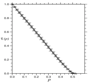
FIG. 1: Strength reduction in a 1602 network due to a random isotropic removal of a fraction p of conductances, averaged over one thousand trials. Numerical results are shown by boxes along with the statistical error, while those obtained by fitting to expres-sion (1) are shown as a continuous line.
(2) the expected size of the largest fracture when elements are removed with a probability pis lnM/ln(1/p). (3) Asp→
pc, the yield strength vanishes asτ(p)→(pc−p)t. Equation (1) is valid throughout the rangep∈[0,pc) [23], and we use it to estimate pcand the critical indext. We then confirm the value oftusing finite size scaling.
The yield current for a given network is computed as fol-lows: given the conductanceσiof all electrical elements in the network and the potentialVoof the top layer of nodes, we use Kirchhoff’s laws to determine the currentsikthrough each element and the potential differencesvk across them. We denote the largest of the latter byVmax. The network will “yield” whenVmaxreachesVb. SinceVmaxandI(p)grow lin-early withV0, the yield current isIyield(p) =I(p)×Vb/Vmax.
III. RESULTS AND DISCUSSIONS
Our computations used networks with sizes M = 20,30,40,50,70,80,90,120,140 and 160, and sample sizes of 10,000 forM=20,30,40,50, sample size of 2,500 for M =70,80,90 and finally sample size of 1,000 for M=120,140,160. Figure 1 shows the behavior ofτ(p)for the 160×160 networks, where the error bars show standard
errors. Although fluctuationsδτinτ(p)decrease asp→pc, the relative fluctuations (δτ/τ) increase. The solid line shown in Figure 1 represents the best fit to Equation (1) with pa-rametersa1,a2,pcandt in a 1602conducting network. To determine their values,a1=−0.1043±0.005,a2=0.061± 0.003,pc=0.513±0.002 andt=1.228±0.015, we used the Lavenberg-Marquadt method to implement the nonlinear fit [37]. We must fittandpcbecause they depend on the size of the network.
0 0.03 0.06 0.09 0.12
x
0.5 1 1.5
t
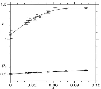
pc
FIG. 2: Variation of parameterst and pcversus the inverse cor-relation length (x=M−0.75), for networks of size M =20 to M=160. All elements in the initial networks have conductance of 1 unit. Note that, both critical values fort(=1.066±0.056)and
pc(=0.500±0.006)are getting in the limit whenx→0.
size. We express the parameters as a function ofx=M−1/ν
whereν(=4/3 for 2D square networks) is the universal cor-relation length exponent [38, 39]; i.e,xis the inverse of the mean size of the largest domain in a network of sizeM×M. Figure 2 shows the values oft(x)andpc(x), along with the error estimates.
We estimate the value of t(0) corresponding to an infi-nite network by first approximatingt(x)by a rational func-tion f(x)/g(x) (where f(x) and g(x) are polynomials of order 3 and 2 respectively) and extrapolating to x= 0. The values of the extrapolation corresponding to Figure 2 are pc(0) =0.500±0.006,t(0) =1.066±0.056,a1(0) =
−0.106±0.015 and a2(0) =0.060±0.004. The error
es-timate includes both errors at each M and those due to the extrapolation [37].
We now validate our results using finite size scaling to in-dependently estimatet(0). According to the finite size scal-ing ansatz, for the correctt(0), the relationship between the rescaled variables τ=Mt(0)/ν×τand ζ=M−1/ν(pc−p) is independent of the system size M[40]. Although the fi-nite size scaling ansatz need hold only for p → pc (and 0<M−1/ν<1), we find that the data collapses to a scaling
functionτ(ζ)over the entire range p∈[0,pc]; see Figure 3 (left side). We then determine the best value fort(0): for any chosen value oft(0), we approximate the scaling function
τ(ζ)by a rational function f(x)/g(x)(where f(x)andg(x) are polynomials of order 3 and 2 respectively) and estimate the deviation of the data(ζk,τk)from the scaling function byχ2=∑
k(τk−τ(ζk))2. Here, the sum is over all available networks. Figure 3 (right side) shows theχ2 as a function oft(0); the best estimate, which we assume minimizesχ2, is tFSS=1.07±0.10, where the error estimate corresponds to doubling theχ2value. This estimate agrees with that value we obtained from Equation (1). These processes are fol-lowed in calculations for other classes of networks discussed
below.
Next we consider networks from which elements are re-moved anisotropically. We begin with a square network of unit conductances and remove elements in the horizon-tal and vertical directions with probabilities ph=βp and pv=p. Analysis of such networks forβ=2.0 using Equa-tion (1) gives pc=0.3383±0003,t=1.33±0.02. Simi-larly, forβ=1/2 , pc=0.68±0.01,t=1.04±0.06 (See Figure 4). Finite size scaling for the two cases estimates give tFSS=1.30±0.10 andtFSS=1.05±0.10 respectively, in good agreement with results obtained from the use of Equa-tion (1). The estimates for pc for multiple β’s, shown in Figure 4, agree with theoretical results for anisotropic net-works [1].
Next, we consider the following process with a two-step degradation. Random removal of conductors is followed by multiplying the conductivity of the remaining conductors by a random number in the range(1−ε,1+ε); whereε∈(0,1).
Note that, the isotropic case is retrieved forε = 0. This process is meant to model age-related changes in trabecu-lar bone. Specifically, while elements of the trabecutrabecu-lar net-work are removed with aging, those remaining can become weaker or stronger - through bone regeneration- depending on the mean loads they carry [15]. We find that the critical index depends on the value ofε. We conduct our analysis for
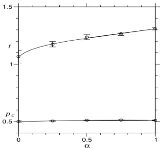
ε=0.00,0.25,0.50,0.75,0.85,0.95 and 1.0, and at eachε, for network sizes considered earlier. Although the value of the critical point pc is independent ofε(Figure 5), and the critical exponent increases withε(forε> 0.5 ) (Figure 5), consistent with results for finite size scaling.
Next, we consider networks where electrical elements that remain in the network are randomly degraded aspincreases. Once again, this problem is related to degradation of porous bone with aging [41], namely the simultaneous loss of tra-becular elements and reductions of the average thickness of the remaining elements. In modeling this dual process, we assume a proportionality between the two types of degrada-tion. Specifically, we consider networks whose conductance and breakdown decrease by a factor(1−αp), where as
be-1.00 1.10 0.0
0.1
-20 -10 0
0 20 40 60
t
ξ
χ
τ 2
FIG. 3: The left side of the figure shows the scaling function (τ) behavior as a function of the network correlation length (ξ), and its
1 2 3 0
0.5 1 1.5
β
pc t
FIG. 4: Values oft(β)andpc(β)withβ, for anisotropic removal of conductance. Elements in the vertical and horizontal directions are removed with probabilitiespandβp.
fore,pis the probability for an element to be removed from the network. Once again, as earlier, we analyzed network sizes ranging fromM=20 toM=160 (Figure 6). Forα= 1.0 we find that pc=0.509±0.005,t=1.29±0.03,a1=
−0.123±0.006 anda2=0.067±0.003. The estimated crit-ical exponent using finite size scaling istFSS=1.29±0.10.
We end this Section by briefly discussing a clinically rele-vant issue. The primary non-invasive diagnostic used to esti-mate bone strength and the need for therapy is bone density [18, 41]. In using it, there is an implicit assumption that the relationship between bone strength and density is indepen-dent of the damage modality of bone. The fact that the
per-0 0.5 1
0.5 1 1.5
pc t
ε
FIG. 5: Behavior oft(ε)and pc(ε)withε, when conductances of the initial network are chosen randomly within(1−ε,1+ε). Bonds
removal is isotropic (pcremains at 0.5).
0 0.5 1
0.5 1 1.5
t
p
α
c
FIG. 6: Variations in parameterst(α)and pc(α). When elements are removed from the network with probabilityp, the conductance of those remaining are reduced simultaneously by a factor(1−αp).
The critical fraction removed elements remain 0.5.
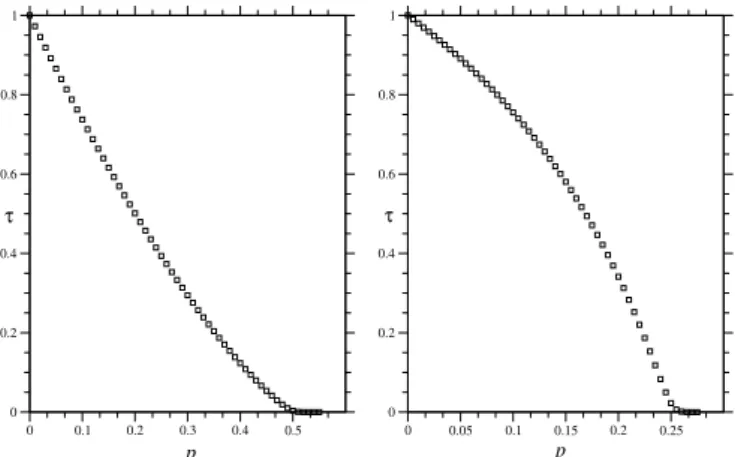
colation threshold and the critical index forτ(p)depend on the modality of damage brings the validity of this assumption into question. To test it, we study two distinct degradations of networks, see Figure 7. The panel on the right shows the
τ(p)for the anisotropic decay withβ=3.0, while that on the left shows the relationship when conductors are randomly removed from the network while the remaining elements are reduced in strength by a factor (1−0.75p). Clearly, the relationship betweenτ(p)andp(and hence very likely the relationship betweenτ(p)and bone density) depends on the damage modality. This observation suggests bone density scans, although widely used, may not be a reliable surrogate for bone strength.
IV. CONCLUSIONS
We have computed percolation threshold pc and critical indextfor square networks of conductances under different damage modalities. These studies are motivated by types of age-related damage in human trabecular bone, and the need to assess their effects on bone strength. The computations are based on the expression (1) which was shown to hold for values of p∈[0,pc)[23]. We validate the values oft using finite size scaling. For isotropic removal of conduc-tances, we foundt=1.07±0.06 in agreement with the value t=1.1 reported by Kirkpatrick [30], Straley [42, 43], and Stinchcombe and Watson [44]. However, it is different from the values obtained using real space renormalization group methods [34, 44–49] and low density series expansion [50– 52]. Series expansion has also been used to compute nu-merically the critical exponent [53], where ford=2 the best estimate ist=1.299±0.002. Many of these discrepancies
have already been discussed by Straley [42].
0 0.1 0.2 0.3 0.4 0.5 0
0.2 0.4 0.6 0.8 1
τ
p
0 0.05 0.1 0.15 0.2 0.25 0
0.2 0.4 0.6 0.8 1
p τ
FIG. 7: The deviation from linearity of the strength reduction due to the removal of a fraction of conductance in a 1602network. The right side shows the anisotropic removal of conductance with prob-abilitiespand 3.0pin the vertical and horizontal direction. The left side corresponds the case where the elements are randomly re-moved with probabilitypmeanwhile the ones remaining are simul-taneously reduced by a factor(1−0.75p).
of experimental and computational results by Han, Lee and Lee [54] and Smith and Lobb [55]. Both groups found that t =1.3 when p=0.33. Figure 4 shows that for p=0.33, the parameter β is 1.94 and t =1.31, in agreement with these previous analyses. Further, the values of pc(β) for anisotropic removal of conductances (Figure 4) is consistent with theoretical results of Redner and Stanley [1].
Perhaps our most interesting observation is the depen-dence of the critical index of the conductance network on the damage modality. It would be of interest to develop a renormalization group analysis to understand this variation. We have, thus far, not been successful in identifying such a theory.
Acknowledgments
The authors would like to thank Dr. K.E. Bassler for use-ful discussions. This work was partially funded by the Na-tional Science Foundation through grants DMS-0607345 and CMMI-0709293, the Institute of Space Science Operations and the ICSC-World Laboratory.
[1] S. Redner and H. E. Stanley, J. Phys. A: Math. Gen.12, 1267 (1979).
[2] S. Redner, Review article for the Encyclopedia of Com-plexity and System Science (Springer Science), in Press, in
arXiv:0710.1105, 27 pages (2007).
[3] M. Sahimi and J. D. Goddard, Phys. Rev. B32, 1869 (1985). [4] J. W. Chung, A. Ross, J. Th. De Hosson and E. van der
Giessen, Phys. Rev. B54, 15094 (1996).
[5] P. Ray and B. K. Chakrabarti, Phys. Rev. B38, 715 (1988). [6] Y. Kantor and I. Webman, Phys. Rev. Lett.52, 1891 (1984). [7] V. K. S. Shante and S. Kirkpatric, Adv. Phys.20, 325 (1971). [8] H. Takayasu, Phys. Rev. Lett.54, 1099 (1985).
[9] J. C. Dyre and Th. B. Schoder, Rev. of Modern Phys.72, 873 (2000).
[10] A. Hansen, E. L. Hinrichsen and S. Roux, Phys. Rev. B43, 665 (1991).
[11] A. Hansen, E. L. Hinrichsen and S. Roux, Phys. Rev. Lett.66, 2476 (1991).
[12] C. Tsallis and S. Redner, Phys. Rev. B28, 6603(R) (1983). [13] Zhenuhua Wu, Eduardo L´opez, Sergey V. Buldyrev, L´ıdia A.
Braunstein, Shlomo Havlin, H. Eugene Stanley, Phys. Rev. E
71, 045103(R) (2005).
[14] Guanlian Li, L´ıdia A. Braunstein, Sergey V. Buldyrev, Shlomo Havlin, H. Eugene Stanley, Phys. Rev. E75, 04501(R) (2007). [15] Y. C. Fung,Biomechanics: Mechanical Properties of Living
Tissue(Springer - Verlag, N. Y., 1993).
[16] K. G. Faulkner, J. Bone Miner. Res.15, 183 (2000).
[17] G. H. Gunaratne, C. S. Rajapakse, K. E. Bassler, K. K. Mo-hanty and S. J. Wimalawansa, Phys. Rev. Lett. 88, 68101 (2002).
[18] E. F. Morgan and T. M. Keaveny, J. Biomech.34, 569 (2001). [19] B. K. Chakrabarti and L. G. Benguigui,Statistical Physics of Fracture and Breakdown in Disordered Systems(Oxford Uni-versity Press, Inc. N. Y., 1997).
[20] P. M. Duxbury, P. D. Beale and P. L. Leath, Phys. Rev. Lett.
57, 1052 (1986).
[21] P. M. Duxbury, P. D. Beale and P. L. Leath, Phys. Rev. B36, 367 (1986).
[22] H. J. Herrmann, A. Hansen and S. Roux, Phys. Rev. B39, 637 (1989).
[23] J. S. Espinoza Ortiz, Chamith S. Rajapakse and Gemunu H. Gunaratne, Phys. Rev. B66, 144203 (2002).
[24] G. H. Gunaratne, Phys. Rev. E66, 061904 (2002). [25] J. W. Esam, Rep. Prog. Phys.43, 53 (1980).
[26] D. Stauffer and A. Aharony,Introduction to Percolation The-ory(Taylor and Francis, London, 1992).
[27] P. M. Duxbury, R. A. Guyer and J. Machta, Phys. Rev. B51, 6711 (1995).
[28] C. J. Lobb and D. J. Frank, Phys. C12, L827 (1979). [29] S. Kirkpatrick, Rev. Mod. Phys45, 574 (1973).
[30] S. Kirkpatrick,Proceeding on the Summer School on III Con-densed Matter(North Holland, Amsterdam, 1978).
[31] Y. Gefen, A. Aharony, B. B. Mandelbrot and S. Kirkpatrick, Phys. Rev. Lett.47, 1771 (1981).
[32] L. Benguigui, Phys. Rev. B34, 8176 (1986).
[33] B. I. Halperin, S. Feng and P. N. Sen, Phys. Rev. Lett.54, 2391 (1985).
[34] D. J. Frank and C. J. Lobb, Phys. Rev. B37, 302 (1988). [35] B. I. Halperin, Physica D38, 179 (1989).
[36] M. Sahimi, Application of Percolation Theory (Taylor and Francis, London, 1994).
[37] W. H. Press, S. A. Teukolsky, W. T. Vetterling and B. P. Flan-nery, Numerical Recipes - The Art of Scientific Computing (Cambridge University Press, 1988).
[38] M. P. M. den Nijs, J. Phys. A12, 1857 (1979).
[39] Yu A. Dzenis and S. P. Joshi, Phys. Rev. B49, 3566 (1994). [40] M. E. J. Newman and G. T. Barkema,Monte Carlo Methods
in Statistical Physics(Oxford University Press, 2001). [41] L. Mosekilde, Bone9, 247 (1988).
[42] J. P. Straley, J. Phys. C10, 1903 (1977). [43] J. P. Straley, Phys. Rev. B15, 5733 (1977).
(1976).
[45] M. Stephen, Phys. Rev. B17, 4444 (1978).
[46] A. B. Harris, S. Kim and T. C. Lubensky, Phys. Rev. Lett.53, 743 (1984).
[47] O. Stenull, H. K. Janssen and K. Oerding, Phys. Rev. E59, 4919 (1999).
[48] J. Bernasconi, Phys. Rev. B18, 2185 (1976).
[49] P. J. Reynolds, W. Klein and H. E. Stanley, J. Phys. C10, L167 (1977).
[50] R. Fisch and A. B. Harris, Phys. Rev. B18, 416 (1978).
[51] J. Adler, J. Phys. A: Math. Gen.18, 307 (1985).
[52] J. Adler, Y. Meir, A. Aharony, A. B. Harris and L. Klein, J. Stat. Phys.58, 511 (1990).
[53] J. M. Normand, H. J. Herrmann and M. Hajjar, J. Stat. Phys.
52, 441 (1988).
[54] K. H. Han, J. O. Lee and Sung-I K Lee, Phys. Rev. B44, 6791 (1991).