Advances in Mechanical Engineering 2016, Vol. 8(5) 1–16
ÓThe Author(s) 2016 DOI: 10.1177/1687814016649300 aime.sagepub.com
Error modeling and tolerance design of
a parallel manipulator with full-circle
rotation
Yanbing Ni, Cuiyan Shao, Biao Zhang and Wenxia Guo
Abstract
A method for improving the accuracy of a parallel manipulator with full-circle rotation is systematically investigated in this work via kinematic analysis, error modeling, sensitivity analysis, and tolerance allocation. First, a kinematic analysis of the mechanism is made using the space vector chain method. Using the results as a basis, an error model is formulated considering the main error sources. Position and orientation error-mapping models are established by mathematical transformation of the parallelogram structure characteristics. Second, a sensitivity analysis is performed on the geo-metric error sources. A global sensitivity evaluation index is proposed to evaluate the contribution of the geogeo-metric errors to the accuracy of the end-effector. The analysis results provide a theoretical basis for the allocation of tolerances to the parts of the mechanical design. Finally, based on the results of the sensitivity analysis, the design of the tolerances can be solved as a nonlinearly constrained optimization problem. A genetic algorithm is applied to carry out the alloca-tion of the manufacturing tolerances of the parts. Accordingly, the tolerance ranges for nine kinds of geometrical error sources are obtained. The achievements made in this work can also be applied to other similar parallel mechanisms with full-circle rotation to improve error modeling and design accuracy.
Keywords
Parallel manipulator, full-circle rotation, error modeling, sensitivity analysis, tolerance allocation
Date received: 4 March 2016; accepted: 18 April 2016
Academic Editor: Jose Ramon Serrano
Introduction
The industrialization of high-speed parallel robots can be greatly promoted by improving their accuracy. As the foundation of accuracy problems, error modeling can provide a theoretical basis for accurate design and kinematic calibration by establishing the mapping rela-tionship between the pose errors in the end-effector and the geometric error sources of the mechanism.
In recent years, a number of error models for paral-lel manipulators have been established. The matrix per-turbation method based on Denavit–Hartenberg (D-H) homogeneous transformation is a classical approach for error modeling.1,2Yao et al.3applied the matrix dif-ferential method to establish a static position and
orientation error model and analyzed their contribu-tions to the pose error of end-effector for a wheeled train uncoupling robot with 4 degrees of freedom (DOF). And the input motion planning method is adopted to improve the position and orientation accu-racy. Wang et al.4 established an error model for a redundant hybrid robot, which had the ability to account for static error sources. However, this method
Department of Mechanical Engineering, Tianjin University, Tianjin, China Corresponding author:
Yanbing Ni, Department of Mechanical Engineering, Tianjin University, Tianjin 300354, China.
Email: [email protected]
has the problem that the parameters become discontin-uous when the adjacent axes are parallel. Thus, many modified approaches have been proposed. Judd5 intro-duced additional parameters into the parallel axis prob-lem and established a modified four-parameter model. However, the corresponding D-H error representation is ill-conditioned when the adjacent axes are vertical. Zhuang et al.6proposed a complete and parametrically continuous model, which is able to avoid mutation of the parameters. Besides this, they pointed out that the change in pose is very small as a result of a change in the parameters. Subsequently, the parameters are guar-anteed to be complete and continuous.
Differential geometry is another powerful tool for modeling errors in parallel manipulators. Tao et al.7 established a kinematic model for robot manipulators using a ‘‘product of exponentials’’ (POE) approach. This has the advantage of avoiding parameter disconti-nuity and also simplifies the calibration process some-what. Using Lie groups and Lie algebra, Chen et al.8 established an error model for a serial robot with 6 DOF according to the transformation principles of Lie algebra. They then integrated the links’ geometric errors and the joints’ offset errors together using the quotient manifold of the Lie group so that all errors could be identifiedsimultaneously.
Recently, ‘‘screw theory’’ has been widely applied to error modeling. Zhao et al.9applied screw theory to a 2-DOF mechanism and simulated a 5-axis blade milling machine. They also applied their method to evaluate the physical effects of the geometric error sources. Coincidentally, Frisoli et al.10adopted screw theory to determine the position accuracy of parallel manipula-tors under the influence of joint clearances. They applied the method to two 3-DOF translational manip-ulators and computed the angular- and linear-positioning accuracy. Kumaraswamy et al.11 adopted screw theory to analyze the kinematic accuracy of mechanisms with varying link lengths and joint clear-ances and demonstrated that it can be applied conveni-ently for closed- or open-loop serial manipulators.
As these matrix methods often involve a large num-ber of matrix differential operations, the vector chain method (based on first-order perturbation theory) is widely used. Briot and Bonev12developed a kinematic error model for a parallel robot to analyze the maxi-mum orientation and position output errors. Cheng et al.13established a pose error model of a symmetrical parallel robot and obtained a statistical model for the sensitivity coefficients. Although the above approaches are widely used for error models, they cannot separate compensatable and uncompensatable error sources. As the pose error of lower-mobility parallel manipulators cannot be compensated,14 these approaches are not suitable for such manipulators. Bearing this in mind, Huang et al.,15 taking a 3-DOF parallel kinematic
machine with parallelogram struts as an example, pro-posed a modeling method to separate the geometric error sources which affect the position and orientation errors in the end-effector. Using the homogeneous transformation matrix method and screw theory, Liu et al.16proposed a general and systematic error model method which allowed the error sources affecting the compensatable and uncompensatable pose accuracy of a platform to be identified in an explicit manner.
Accuracy analysis is a powerful method of mitigat-ing uncompensatable error. For a 6-DOF parallel mechanism, Patel and Ehmann17 proposed an error model that divides the error sources into those affecting leg lengths and those affecting joint positions. Then, the tolerance allocations of the parts were studied with the aid of a sensitivity analysis. Wang and Ehmann18 presented first- and second-order error models for a 6-DOF Stewart platform. By means of a sensitivity analysis, the contribution of each error component to the total position and orientation error of the mechan-ism was thus determined. Kim and Choi19proposed an ‘‘error range’’ method, which established a relationship between the pose error of the end-effector and the pose errors of the joint. This was then used to instruct toler-ance allocation. Soon et al.20 constructed an error-mapping model for a Hexapod based on the vector chain method. In this work, a sensitivity analysis was again applied to analyze the errors. Together with the aid of an experiment that measured errors, this work’s results suggest that the pose error is equal to the mean value of each error source. Chen et al.21established an error model for a novel ‘‘selective compliance assembly robot arm’’ parallel robot with parallelogram struc-tures. The model was able to reflect the process of error transmission in detail and show the influence of each geometric error on the pose error of the moving plat-form via a sensitivity analysis. Maurine and Domber22 proposed an error-mapping model for a mechanism with characteristic parallelogram structures and used the result of a sensitivity analysis to estimate the pose accuracy of the end-effector. Although the above approaches are widely used in accuracy analyses, they cannot filter out the effect of uncompensatable error sources on pose accuracy. For a translational parallel mechanism with parallelogram struts under constraint, Huang and colleagues23,24 considered that the relative and coplanar errors of the parallelogram have a uncompensatable effect on the pose of the end-effector. In order to reduce these two kinds of errors, they sub-sequently proposed an assembly process which was effectively able to suppress the pose error of the end-effector.
parallel mechanisms. In addition, they do not propose a comprehensive and universally applicable method of integrating error analysis and accuracy design into lower-mobility parallel mechanisms. This article con-siders a novel parallel manipulator with full-circle rota-tion. The novel manipulator enables kinematic analysis, error modeling, sensitivity analysis, and toler-ance allocation to be integrated into a comprehensive framework. Therefore, the work presented addresses the disadvantages of the methods in the literature dis-cussed above by separating pose errors, determining the influence of each error on the pose accuracy of the end-effector, and reducing the uncompensatable error. The method provides tolerance ranges for the uncom-pensatable error sources which are required in the man-ufacturing and assembling stages with the aid of a sensitivity analysis.
The work of this article is organized as follows. Section ‘‘Kinematic analysis’’ describes the manipulator system and presents an inverse kinematics analysis, which provides the foundation for the rest of the work. Section ‘‘Error-mapping model and error separation’’ establishes an error model for the manipulator based on the vector chain method. Then, the position and orientation error sources that affect the accuracy in the end-effector are effectively separated by application of a mathematical transformation with parallelogram structure characteristics. Section ‘‘Sensitivity analysis’’ adopts a global sensitivity evaluation index to carry out a sensitivity analysis of all the error sources. The law governing the effect of the geometric parameter errors
on the accuracy in the end-effector is proposed, which lays the foundation for the subsequent work on accu-racy design. Section ‘‘Tolerance allocation’’ performs tolerance allocation using a genetic algorithm (GA), which provides fundamental guidelines for component manufacture and assembly. Section ‘‘Conclusion’’ pre-sents the conclusions of this article.
Kinematic analysis
System description
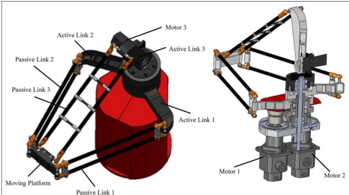
The object considered in this study is shown in Figure 1. The parallel manipulator with full-circle rota-tion,25,26 which has two translational and one rota-tional (2T1R) DOF, consists of a fixed frame, servo motors, three branched chains, and a moving platform. In the first and second chains, the active links are con-nected to their servo motors by a transmission mechan-ism, but in the third chain, the active link is directly connected to the servo motor. One end of each passive link is connected to its active link by a spherical joint, while the end side is connected to the moving platform. A parallelogram structure is employed in each passive link. To ensure the follow-up characteristic, the passive link of the third chain is fixed using three tie rods that are equal in length to a rod that contains the revolute joints on both sides. The third chain can realize two-dimensional translations on thex2o2z2 plane and rota-tion about z2-axis (Figure 2). All three chains contain revolute joints that rotate around the same axis, and all the ends of the passive links are connected to the
moving platform. Thus, one translation and two rota-tions are realized and a larger workspace and broader transmission range acquired.
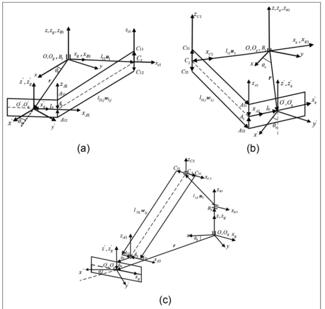
A schematic diagram of the parallel manipulator with full-circle rotation is shown in Figure 2. We take the coaxial hinge point of active links 1 and 2 as the origin Oand their coaxial rotation axis as the Z-axis. As the manipulator can realize full-circle rotation, the X- andY-axes can be selected randomly following the right-hand rule. A fixed coordinate system OXYZ can thus be established and all vectors described within the OXYZ frame. Rotating byu0 around the Z-axis of the fixed coordinate system in a counterclockwise direction, the moving coordinate system o1x1y1z1 is established. In the axis hinge point of active link 3, we also establish the moving coordinate systemo2x2y2z2 with o2 being the origin and z2-axis being coincident with theZ-axis. Thex2-axis is in the direction of rota-tion axis of active link 3, and the y2-axis is defined by the right-hand rule. The moving coordinate system o2x2y2z2can be obtained by rotating the frame antic-lockwise about theZ-axis byu0+p=2.
Inverse kinematic analysis
Inverse kinematic analysis27 is considered to determine the active link position angleui(i=1,2,3) (the range of
u1 and u3 is 0p, and the range of u2 is p2p) according to the position vectorr= (x y z)T of the
reference pointAon the moving platform (which is2l0 and 2b0 in the length and width directions, respec-tively). The offset displacement of kinematic chain 3 is h along the direction of the z-axis. The distance between the location of the center of chain 3 and the
external end-surface of the moving platform is s. The projection of the position vector r= (x y z)T is
u0= ( cosu0 sinu0 0)T on the OXY plane. u0 is the angle between the projection and the positive direc-tion of the x-axis in the coordinate system OXYZ and may be determined from arctan(y=x) =u0.
Inverse kinematic analysis of chains 1 and 2. As chains 1 and 2 have the same structure and form of motion, we can consider them together. In the moving coordinate system o1x1y1z1, u1 is defined as the angle between the active link 1 and the positive direction of the x1-axis,u2 is the angle between the active link 2 and the positive direction of the x1-axis. Thus, uo1
1 = ½cosu1 sinu1 0T, u2o1=½cosu2 sinu2 0T are measured in the moving coordinate systemo1x1y1z1.
In the fixed reference coordinate system, the closed-loop vector equation of chains 1 and 2 can be written as
rl1u1+l0uv=l2wi ð1Þ
wherel1,l2,ui,wi represent the length and unit vector of the active and driven arms of chain i(i=1,2),
respec-tively, andu1= ( cosu0cosu12sinu0sinu1 sinu0cosu1 + cosu0sinu1 0)T,wi= ( cosai cosbi cosgi)T.
The vector uv= (sinu0 cosu0 0) is the normal vector of the projectionron theOXY plane.
Taking the modulus of both sides of equation (1) gives
Aisinui+Bicosui+Ci=0 ð2Þ
where
Ai=2l1xsinu02l1ycosu0+ (1)i2l0l1
Bi=2l1xcosu02l1ysinu0
Ci=x 2
+y2+z2+l21l 2 2+l
2 0
+ð1Þi2l0ðxsinu0+ycosu0Þ
According to the assembly mode, inverse position analysis gives
ui=2arctan Ai+
ffiffiffiffiffiffiffiffiffiffiffiffiffiffiffiffiffiffiffiffiffiffiffiffiffiffiffiffi
A2 i C
2 i +B
2 i
p
CiBi
ð3Þ
Accordingly, ui can be determined. In addition, wi
can be determined from
wi=rl1ui+ (1)
i+1 l0uv l2
ð4Þ
Inverse kinematic analysis of chain 3. Here, we establish a reference coordinate system o2x2y2z2 for chain 3 involving rotating around theZ-axis of the fixed coordi-nate system in a counterclockwise direction byu0+p=2.
The z2-axis coincides with the Z-axis of OXYZ, the rotation axis of the active link 3 is thex2-axis, and the y2-axis is vertical according to the right-hand rule (Figure 2). We defineu3as the angle between the active link 3 and the positive direction of thex2-axis.
Next, we define the vector uo2
3 = (0 cosu3 sinu3)T. Transformation ofuo2
3 into the fixed coordinate system OXYZ yields the vectoru3= (cosu0 cosu3 sinu0 cosu3 sinu3)T and the closed-loop vector equation for chain 3 can be written as
rl1u3he0+b0e0su0=l2w3 ð5Þ
where e is the offset of the kinematic chain 3 with e0=he0ande0is a unit vector the alongZ-axis.
The following trigonometric expression is obtained by taking the modulus of both sides of equation (5)
A3sinu3+B3cosu3+C3=0 ð6Þ
where
A3 ¼2l1xsinu02l1ycosu0þ ð1Þi2l0l1 B3 ¼ 2l1xcosu02l1ysinu0
C3 ¼x 2
þy2þz2þl21l 2 2þl
2 0
þ ð1Þi2l0ðxsinu0þycosu0Þ
Considering the assembly mode gives the solution
u3=2arctan A3+
ffiffiffiffiffiffiffiffiffiffiffiffiffiffiffiffiffiffiffiffiffiffiffiffiffiffiffiffi
A2 3C
2 3+B
2 3
p
C3B3
ð7Þ
Thus,u3can be determined andw3can then be
deter-mined from
w3=rl1u3he0+b0e0su0
l2
ð8Þ
Note thatu1 andu2 values obtained should be added (u0= ((u01+u
0
2)=2)p). Then, they are changed into
u01=u1+u0,u02=u2+u0. They are the driven angle of the active arm with respect to the fixed coordinate system.
Error-mapping model and error
separation
Description of the coordinate systems and error
analysis
There are some structural similarities between the par-allel manipulator with full-circle rotation and existing parallel manipulators with parallelogram strut struc-tures.28Therefore, the following coordinate systems for the parallel manipulator with full-circle rotation can be defined (see Figure 3):
fOg is defined with reference to the machine frame. The originOis the point at which the active link ideal
axis crosses thexyplane which passes through the mid-point of the two joints associated with the active link and which is normal to the line passing through the centers of the two joints.Ois located in thexyplane.
uois the angle between the projection of position vector
ronto thexyplane and thex-axis. They-axis is defined
by the right-hand rule. The angle of the intermediate coordinate system fOgg relative to fOg is uo+p=2 through thez-axis.
fBig is defined with reference to the active links. For i=1,2, Bi is the point of intersection of a vertical line
fromCi on the active link to the actual axis ZBi of the relevant revolute pair. ThexBi-axis is parallel to thexy
plane and theyBi-axis is then defined according to the
right-hand rule. Wheni=3,B3is the intersection point fromC3 on the active link to the corresponding actual axis. ThexB3-axis is coincident with the axis of the
revo-lute pair of the active link. TheyB3-axis is parallel to the
xyplane. ThezB3-axis is defined according to the
right-hand rule.
fCigis placed on the spherical joint of the active link. Wheni=1,2, the origin isCi. ThezCi-axis is coincident
with a line connecting the centers of the corresponding two spherical pairs. The xCi-axis is parallel to the xy
plane. The yCi-axis is defined by the right-hand rule.
Wheni=3, the origin isC3. ThexC3-axis is coincident
with a line connecting the centers of the corresponding two spherical pairs. The zC3-axis is vertical to the xy
plane. TheyC3-axis is defined by the right-hand rule.
fAigis placed on the spherical joint of the passive link. The originAiis the midpoint of the line connecting the moving platform with the line of centers of two spherical pairs of passive links. Wheni=1,2, thezAi-axis is coincident with
the line connecting the centers of two spherical pairs. The xAi-axis is parallel to the xyplane. TheyAi-axis is defined
by the right-hand rule. Wheni=3, thexAi-axis is
coinci-dent with the line connecting the centers of two spherical pairs. TheyA3-axis is parallel to thexyplane. Thel2-axis is defined by the right-hand rule.
fO0gis placed on the moving platform with the origin pointO0 being the point where the center line crosses the ligature of the right and left spherical joints that connect the moving platform and thez-direction verti-cal plane of the moving platform. Thex0y0plane is par-allel to the moving plane of the upper and lower active links. Thex#-axis is parallel to the x-axis, and the y# -axis can be defined by the right-hand rule. The inter-mediate coordinate system fO0
gg can be defined by rotatingfO0gabout thez#-axis byu
o+p=2.
The errors can be described as follows. In chaini, the theoretical value ofBi, which is the position vector of the point infOg, and its error are given by bi (the
fBig, the theoretical value of the unit vector ui from point Bi to point Ci and its error are given byuio and
Dui, respectively. The theoretical value of the length
BiCi=l1iand its error are given byl1iandDl1i, respec-tively. The theoretical value ofwij, which is the unit
vec-tor of link jin the passive link, and its error are given by wi and Dwij, respectively. The theoretical value of
the length l2ij and its error are given by l2i and Dl2ij, respectively. InfO0g, the theoretical value of the length vector of the moving platform and its error are given bylo andDlo, respectively. The theoretical value of the
width vector of the moving platform and its error are given bybo andDbo, respectively. The theoretical value
of the height vector of the moving platform and its error are given bysoandDso, respectively. The
theoreti-cal value ofcij, which is the distance of pointCito the centerCij of the spherical joint, and its error are given
by e=2 and Dci, respectively. The theoretical value of
aij, which is the distance of pointAito the centerAijof the spherical joint, and its error are given by e=2and Dai, respectively. The orientation error vector offO0g referenced tofOgis given byu.
Error-mapping model
According to the definitions of the coordinate systems and the description of the geometric error sources, in the kinematic chain OBiCiCijAijAiO0, the position vector r(see Figure 3) of pointO0 can be expressed infOgby15,26
r=ROO
g ROB1 l11u1+ð1Þ
j+1 RB
1C1c1je3
+l21jw1jROO0RO0O0 g
l0+ð1Þj+ 1
RO0A1a1je3
ð9Þ
r=ROO
g ROB2 l12u2+ð1Þ
j+1
RB2C2c2je3
+l22jw2j
ROO0RO0O0
g l0+ð1Þ j+1
RO0A2a2je3
ð10Þ
r=ROO
g b3+ROgB3 l13u3+ð1Þ
j+1
RB
3C3c3juv
+l23jw3j
ROO0RO0O0
g s0b0+ð1Þ j+1
RO0A3a3juv
ð11Þ
Considering the first-order linear perturbations on both sides of the above equation, we have
Dr=Rg Db1+uB13 l11u1+ð1Þ
j+1 e=2e3
+Rg Dl11u1+uC13ð1Þ
j+1
e=2e3+ð1Þj+ 1
Dc1e3
+ Dl21jw1+l21Dw1j
u3Rgl0+ð1Þj+1e=2e3
Rg Dl0+uA13 ð1Þ
j+1 e=2e3
+ð1Þj+1Da1e3
ð12Þ
Dr=Rg Db2+uB23 l12u2+ð1Þ
je=2e
3
+Rg Dl12u2+uC23ð1Þ
je=2e
3+ð1ÞjDc2e3
+ Dl22jw2+l22Dw2j
u3Rg l0+ð1Þje=2e3
Rg Dl0+uA23 ð1Þ
je=2e
3
+ð1ÞjDa2e3
ð13Þ
Dr=Rg Db3+uB33 l13u3+ð1Þ
j+1 e=2uv
+Rg Dl13u3+uC33ð1Þ
j+1
e=2e1+ð1Þj +1
Dc3e1
+ Dl23jw3+l23Dw3j
+u3Rg s0b0 ð 1Þj+ 1
e=2uv
Rg Ds0+Db0+uA33ð1Þ
j+1
e=2uv+ð1Þj+1
Da3uv
ð14Þ
where
i=1,2,3, j=1,2, e3=ð0 0 1ÞT
Rg is the orientation matrix of Og referenced to O (O0
g referenced toO0) and is given by
Rg=
cosðu0+p=2Þ sinðu0+p=2Þ 0 sinðu0+p=2Þ cosðu0+p=2Þ 0
0 0 1
2
4
3
5
uBk(k=1,2,3) is the orientation error vector ofBk referenced toOg.
uCk(k=1,2,3) is the orientation error vector of Ck referenced toBk.
uAk(k=1,2,3) is the orientation error vector ofAk referenced toO0g.
Let Dai=Dl0(i=1,2), Dai=Ds0+Db0, i=3 be the comprehensive error vector of the origin of Ai
referenced to O0g; c3=uBi+uCiuAi be the orienta-tion error ofO0g referenced toOg;Dgi= 2(DciDai) the relative joint distance error on both sides of the parallelogram and take the product ofwT
i on both sides of equations (12) - (14). Then, we have
wT
1Dr= (w
T
1RgDb1+wT1RgDa1+Dl11wT1Rgu1+l11Rgu13w1
T
RguB1)
+ð1Þj+1
e=2Rge33w1
TR
gc1+Dg1=2w
T
1Rge3
+Dl21j Rg l0+ð1Þj+ 1
e=2e3
3w1 T u ð15Þ wT
2Dr=wT2RgDb2+wT2RgDl0+Dl12wT2Rgu2+l12 Rgu23w2
T
RguB2
+ð1Þj+1
e=2Rge33w2
T
Rgc2+Dg2=2wT2Rge3
+Dl22j Rg l0+ð1Þj+ 1
e=2e3
3w2 T u ð16Þ wT
3Dr=w
T
3RgDb3+wT3RgDa3+Dl13wT3Rgu3+l13 Rgu33w3
TR
guB3 +ð1Þj+1
e=2Rguv3w3
T
Rgc3+Dg3=2w
T
3Rguv
+Dl23j Rg s0+b0+ð1Þ
j+1 e=2uv
3w3
T
u
ð17Þ
It can be seen that the position and orientation errors in the parallel manipulator with full-circle rota-tion are coupled. Note that the orientarota-tion errors can-not be compensated for as the parallel manipulator with full-circle rotation only has three controllable DOFs (associated with one translation and two rota-tions of the platform). Therefore, it is necessary to sep-arate the orientation and position error sources which affect the accuracy in the end-effector from the sources of pose error. In order to achieve the requirement of accuracy in the end-effect, an accuracy analysis and kinematic calibration should be made of the different error sources.
Error separation
Taking the difference between the two closed-loop equations for chains 1, 2, and 3 yields
e Rge33w1
T
u=Dld1+Dg1wT1Rge3
+e e33 RTgw1
T
c1
ð18Þ
e Rge33w2
T
u=Dld2+Dg2wT2Rge3
+e e33 RTgw2
T
c2
ð19Þ
e Rguv3w3
T
u=Dld3+Dg3wT3Rguv
+e uv3 RT
gw3
T
c3
ð20Þ
Rewriting equations (18)–(20) in matrix form leads to the orientation error-mapping function
u=Jueu ð21Þ
Ju=A1B
where
A=e½Rge33w1 Rge33w2 Rguv3w3T
B=diag½ Bi
B1= 1 wT1Rge3 e e33 RTgw1
T
B2= 1 wT2Rge3 e e33 RTgw2
T
B3= 1 wT3Rguv e uv3 RT
gw3
T
eu= eT
u1 eTu2 eTu3
T
eui= Dldi Dgi cT i
T
It is clear that there are three kinds of geometrical error sources affecting the pose accuracy of the end-effector. These include the relative length errorsDldi of the parallelogram, the relative errors Dgi of the dis-tances between the centers of two spherical pairs, and the orientation errors ci of O0g referenced to Og. The errors ci are caused by errors made during assembly. Also, as (e33(RTgw1))?e3, (e33(RTgw2))?e3, the pro-jection of c1z onto (e33(RTgw1)) and c2z onto (Rge33w2) are both zero. This means thatc1zandc2z have no effect on the orientation accuracy of the end-effector. Therefore, it is reasonable to remove the col-umns ofJu associated withc1
z andc2z. As a result, it can be concluded that 13 geometric errors are responsi-ble for the orientation accuracy of the manipulator, and the most important ones are Dldi, Dgi, c1x, c1y, c2x,c2y,c3x,c3y, andc3z.
Additionally, the two closed-loop equations belong-ing to each chain give
wT1Dr=Dla1+wT1RgDb1+wT1RgDa1+Dl11wT1Rgu1
+l11 u13 RTgw1
T
uB1 Rgl03w1
T
u
ð22Þ
wT2Dr=Dla2+wT2RgDb2+wT2RgDa2+Dl12wT2Rgu2
+l12 u23 RTgw2
T
uB2 Rgðl0Þ3w2
T
u
ð23Þ
wT3Dr=Dla3+wT3RgDb3+wT3RgDa3+Dl13wT3Rgu3
+l13 u33 RTgw3
T
uB3 Rgðs0b0Þ3w3
T
u
ð24Þ
whereDlai= (Dl2i1+Dl2i2)=2is the mean of the length errors of the passive link in theith parallelogram chain structure.
Rewriting equations (22)–(24) in matrix form gives the position error-mapping function
Dr=Jrer=½Jrr Jru½err euT ð25Þ
where
Jrr=C1D
Jru=C1E
C=½w1 w2 w3T
D=diag½Di
D1= 1 wT
1Rg wT1Rg wT1Rgu1 l11 u13 RTgw1
T
D2= 1 wT2Rg wT
2Rg wT2Rgu2 l12 u23 RTgw2
T
D3= 1 wT3Rg wT3Rg wT3Rgu3 l13 u33 RTgw3
T
E= ½Rgl03w1 Rgðl0Þ3w2 Rgðs0b0Þ3w3T
err= eT
r1 eTr2 eTr3
T
eri= Dl
ai DbTi DaTi Dl1i uTBi
T
Therefore, the geometrical error parameters affect-ing the position accuracy of the end-effector can be described as: the mean value of the length errors of two passive links of the parallelogram (Dldi), the synthetic error vectors of the originBi relative to the coordinate system O0g(Dbi), the length errors of the active links
(Dl1i), and the orientation errors of Bi relative to the coordinate systemOg(uBi,i=1,2,3). These include the error sources affecting pose accuracy. When the corre-sponding coefficients of two kinds of error sourcesDbi
and Dai are proportional, the corresponding Di col-umns are linearly related. Hence, these two kinds of error sources can be attributed to a class. At the same time, because the error source Db3x on chain 3 has no effect on the accuracy of the end-effector, Jrr needs to
end-effector, including 13 kinds of orientation errors that affect the orientation accuracy of the end-effector.
Sensitivity analysis
Sensitivity analyses can guide tolerance design and assembly of every part by evaluating the degree of influ-ence of the geometrical errors on the orientation accu-racy of every part of the structure. Using a sensitivity analysis, the laws governing the effects of geometric parameter errors on the orientation error of this manip-ulator (with full-circle rotation) can be proposed.
Consider the position error-mapping model
Dr=Jreras an example. The probability model for the
sensitivity analysis is first constructed. Arranging Jr
and er in the order of the chains, the above equation
can be rewritten as
Dr=J0
re 0
r ð26Þ
Taking the norm of both sides of equation (26) yields
Dr2 r=
X
3
i=1
X
3
j=1
Xn
k=1
Xn
l=1
X
3
m=1
J0 rimkJ 0 rjml ! e0 rike 0 rjl ð27Þ
wheree0
rikis thekth element ine0ri,J 0
rimk is the element in rowmand columnkofJ0
ri, andnis the number of geo-metric error parameters in all chains.
We assume that all elements in e0
r are independent random variables and have normal distributions with zero mean. As a result, the mean value ofDrr is zero and
DðDrrÞ=E Dr 2 r
½EðDrrÞ 2
=E Dr2 r
= X
n
k=1
X
3
i=1
X
3
m=1
J02
rimk
!
E e02 rik
, n=12 ð28Þ
For the new manipulator with full-circle rotation, the geometrical errors of the same type in each chain share the same variance, that is
E e02 rk
=E e02 r1k
=E e02 r2k
=E e02 r3k
ð29Þ
Thus, the standard deviation ofDrrcan be expressed as
sðDrrÞ=
ffiffiffiffiffiffiffiffiffiffiffiffiffiffiffiffiffiffiffiffiffiffiffiffiffiffiffiffiffiffiffiffiffiffiffiffiffiffiffiffiffiffiffiffiffiffiffiffiffiffi
Xn
k=1
X
3
i=1
X
3
m=1
J02
rmiks 2 e0
rk v u u t ð30Þ
For the orientation error u= (ux uy uz)T, the standard deviation ofdaanddfcan be expressed as
s dð Þa =
ffiffiffiffiffiffiffiffiffiffiffiffiffiffiffiffiffiffiffiffiffiffiffiffiffiffiffiffiffiffiffiffiffiffiffiffiffiffiffiffiffiffiffiffiffiffiffiffiffiffi
Xn
k=1
X
3
i=1
X
2
m=1
J2
umiks 2
euk ð Þ
v u u
t ð31Þ
s df
=
ffiffiffiffiffiffiffiffiffiffiffiffiffiffiffiffiffiffiffiffiffiffiffiffiffiffiffiffiffiffiffiffiffiffiffiffiffiffiffiffi
Xn
k=1
X
3
i=1
J2
u3iks 2 e uk ð Þ v u u t ð32Þ
Similarly, the sensitivity coefficients of the orienta-tion error with respect to geometric error euk can be expressed as
m0kr=
ffiffiffiffiffiffiffiffiffiffiffiffiffiffiffiffiffiffiffiffiffiffiffiffiffiffi
X
3
i=1
X
3
m=1 J02
rimk
v u u
t , k=1,2,. . .,12 ð33Þ
mak=
ffiffiffiffiffiffiffiffiffiffiffiffiffiffiffiffiffiffiffiffiffiffiffiffiffiffiffi
X
3
i=1
X
2
m=1
J2
uimk
v u u
t , k=1,2,. . .,13 ð34Þ
mfk=
ffiffiffiffiffiffiffiffiffiffiffiffiffiffiffiffiffi
X
3
i=1
J2
ui3k
v u u
t , k=1,2,. . .,13 ð35Þ
These sensitivity coefficients represent the standard deviations of the errors in the end-effector caused by a unit standard deviation of geometrical error. As sensi-tivity coefficients vary with the configuration of the mechanism, their mean values can be employed as a sensitivity evaluation index in the overall prescribed workspace. The index can be defined as
m0kr=
ð
V
m0krdV
0
@
1
A=V, k=1,2,. . .,12 ð36Þ
m0ak=
ð
V
makdV
0
@
1
A=V, k=1,2,. . .,13 ð37Þ
m0fk=
ð
V
mfkdV
0
@
1
A=V, k=1,2,. . .,13 ð38Þ
whereVis the volume of the prescribed workspace. Note that this parallel manipulator can realize full-circle rotation and has the same performance in all direc-tions. As shown in Figure 4, the reachable workspace of reference point on moving platform is the intersection of three subspaces associated with three kinematic chains. The subspace of each chain is the region encircled by three surfaces whose circle center isAi and radius isl2, when active links reach their minimum limits Lmin and
maximum limits Lmax, respectively. According to the
workspace is in the upper part of the reachable work-space as far as possible. The inner boundary of the task workspace is tangent to the inner boundary which is con-straint by the angle (b3=408) of active and passive links 3. The outer boundary of the task workspace is tangent to the outer boundary which is constraint by the angles (b1=b2= 1408) of active and passive links 1 and 2.
Thus, the three global sensitivity evaluation indices above can be measured in the prescribed working area in theyzplane, that is
mkr=
ð
S
m0krdV
0
@
1
A=S, k=1,2,. . .,12 ð39Þ
mak=
ð
S
makdV
0
@
1
A=S, k=1,2,. . .,13 ð40Þ
mfk=
ð
S
mfkdV
0
@
1
A=S, k=1,2,. . .,13 ð41Þ
A sensitivity analysis can be carried out on the par-allel manipulator with full-circle rotation by utilizing the indices given in equations (39) - (41). The nominal dimensions used in the analysis are shown in Table 1. According to the working and force-transfer character-istics of the mechanism, the prescribed workspace is a cylindrical ring with an inner radius of 300 mm, outer radius 650 mm, and height 200 mm. In the yz plane, it is a rectangle, 300 mm away from the central axis, with a length of 350 mm and width of 200 mm (as shown in Figure 4).
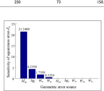
Figures 5–8 show the results of global sensitivity analyses of the pose and volumetric errors da,df, and dr with respect to the geometrical error parameters. As shown in Figure 5, in chains 1 and 2, the orientation geometric errorsDld1 andDld2 have a marked effect on the verticality error da (the spindle axis with respect to
thexyplane). However, in chain 3, the rotational axis of the active link 3 is vertical to the spindle of the mechanism. So, it is on the non-sensitivity direction of error for da. Therefore, the sensitivity coefficients of
the geometric errors in chain 3 with respect to error in the verticality of the spindle axis about thexyplane are zero, such asDld3,Dg3,c3x,c3y, andc3z. It illustrates that some uncompensatable errors will not affect the corresponding orientation errors of the end-effector. Figure 4. Cross-section of the workspace of the parallel
manipulator with full-circle rotation (through theyzplane): (a) Geometric parameters in task workspace and (b) Sectional view of reachable and task workspace.
Figure 5. Sensitivity analysis of the geometric errors with respect to error in the verticality of the spindle axis about thexy plane(i=1,2).
Table 1. Nominal dimensions of the parallel manipulator with full-circle rotation (the linear unit is mm).
l1 l2 b0 s0 l0 b3
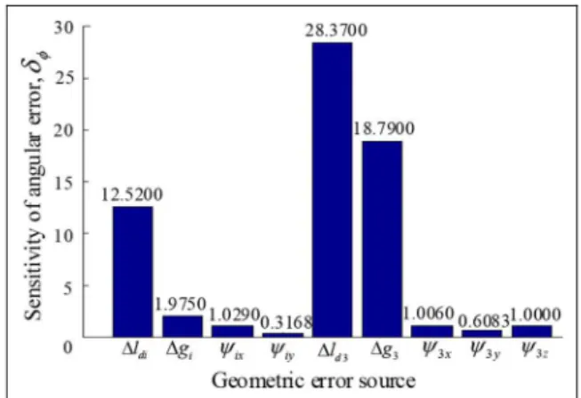
As shown in Figure 6, the geometric parameter error
Dldi has a large effect on the angular error df (about
the z-axis), and the geometric error Dg3 also has an obvious effect on the angular error df (about the
z-axis). If error df due to Dldi is restricted to within 20mm, in accordance with the3sprinciples, the
toler-ance of ldi must be held to T(Dld1) =T(Dld2) =6(3320=12:52) =64:79mm and T(Dld3) =
6(3320=28:37) =62:11mm. The position
geometri-cal errors are sensitive to geometric parameter errors
Dldi, Dlai, Dby, and Dl1i, and the angular geometrical errors are not as sensitive as the linear geometric errors are to position geometrical errors. Similarly, the toler-ance of Dlai must be T(Dla1) =T(Dla2) =6(3320=
1:953) =630:72mm=m and T(Dla3) =6(3320=
1:482) =640:48mm=m.
Tolerance allocation
For the parallel mechanism with less freedom, the uncompensatable error sources cannot be compensated for by kinematic calibration. In order to guarantee the accuracy in the position and pose of the mechanism, the manufacturing tolerances of the parts need to be suitably allocated via tolerance optimization. There are nine kinds of geometric error sources for the parallel manipulator with full-circle rotation. In order to reduce the manufacturing cost, the tolerance of the geometric parameters should be relaxed as far as possible subject to the premise that the tolerances of the orientation errorsda and df are less than the allowable values in
the global workspace. Thus, we assume that the nine kinds of uncompensatable error sources are design variables and that the tolerance manufacturing cost is the objective function. Then, giving the required toler-ance range of the two errors da, df and taking each
error source as the constraint factors, the tolerance design of each component is converted into a nonli-nearly constrained optimization problem, as follows
minf= X 9
k=1 sk
s2 (De0
ck)
ð42Þ
wheresk are the process parameters which, for length and angle parameters are, respectively, 1 and 1.5
maxðs dð Þa Þ ½s dð Þa
max s df
s df
inf s De0 ck
s De0 ck
sup s De0 ck
8
<
:
ð43Þ
where max(s(da)) is the maximum of the standard
deviation of the squareness error in the end-effector; max(s(df)) is the maximum of the standard deviation
of the spindle angular error; ½s(da) is the maximum
allowable value of the standard deviation of the square-ness error in the end-effector; ½s(df)is the maximum
allowable value of the standard deviation of the spindle angular error; sup(s(De0
ck)) is the upper limit of the standard deviation of the uncompensatable error Figure 6. Sensitivity analysis of the geometric errors with
respect to the angular error in thez-axis(i=1,2).
Figure 7. Sensitivity analysis of the geometric error with respect to position error in chaini(i=1,2).
sources; and inf(s(De0
ck)) is the lower limit of the stan-dard deviation of the uncompensatable error sources.
This is a complicated optimization problem, one which we tackle using a GA. GA is an evolutionary algorithm. It is based on imitating the mechanism of genetic selection that occurs in nature to find the opti-mal solution.
GA includes three basic operators: selection, cross-over, and mutation. First, the algorithm searches for a set of approximate optimal values among all the possi-ble values, which then form the genetic population. Then, it screens for satisfactory individuals among the genetic group to form a new population. In the screen-ing process, new individuals are continuously produced by crossover and mutation. Finally, a set of satisfactory optimal values are obtained. Iteration is the main numerical process used to solve this nonlinear optimi-zation problem. However, iterative methods in general can easily fall into local minima which may trap them, and as a result, the phenomenon referred to as ‘‘death cycle’’ is observed. GA is capable of overcoming this shortcoming. As a consequence, a GA is better placed to find the global minimum error. Moreover, compared with other optimization methods, GA that has small population sizes and high mutation rates can rapidly find a good solution.
In this work, the solution process is directly per-formed using the GA toolbox built into the MATLAB
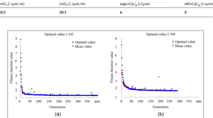
software application. The minimum value of the objec-tive function is the fitness function, which is determined by equation (39). The constraint conditions are deter-mined using equation (40). Table 2 shows the allowable parameter values wherein the standard deviations are determined as per JB/T 10792.1-2007.29
Parameters needed to implement the GA include variable dimensions, number of generations, population size, mutation probability, and crossover probability. In this case, the variables are nine kinds of uncompen-satable error sources and so the variable dimension is 9. The number of generations is taken to be 400, which can produce good calculated values and is relatively fast. Figure 9 shows the optimization process when the population size is set to 20 and 80, both of which have bad convergences. Using a large population size has the advantage of improving the search quality of the GA and prevents convergence before maturation. However, it also increases the number of calculations involved and reduces the rate of convergence.
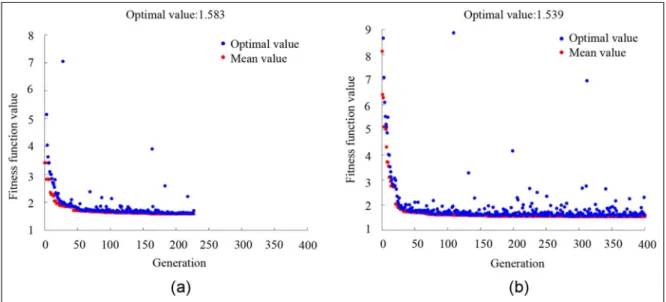
Figure 10 shows the optimization processes when the crossover probability is set to 0.05 and 0.99. When the crossover probability is large, the introduction of a new structure is more likely. However, it also results in ran-domization. A low crossover probability may make the genetic search stagnate.
Figure 11 shows the optimization processes when the mutation probability is set to 0.001 and 0.08. Mutation Table 2. Allowable parameter values.
½s(da)(mm=m) ½s(df)(mm=m) sup(s(De0
ck)) (mm) inf(s(De0ck)) (mm)
40/3 30/3 6 0
probability is an important factor that keeps the popu-lation diverse. A low mutation probability may easily generate a local extreme value, but too a high mutation probability can make the genetic search too random. Mutation probability affects the ability of the algorithm to search locally, whereas the crossover probability affects the ability of the algorithm to search globally. So, they need to be coordinated with each other in an appropriate manner.
The selection of the parameters discussed above is dependent on the type of problem involved. Therefore, in any actual problem, one needs to change these
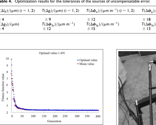
parameters continuously in order to obtain the best results according to certain requirements. The above selection process is appropriate in special situations. Actually, in the current situation, many simulations have been done that suggest the best values to use. The final parameter values assumed are shown in Table 3. The values of the fitness function subsequently obtained using the GA are shown in Figure 12.
Based on the3s criterion, the standard deviation of
each geometric error source is transformed into a toler-anceT=63s. The results are shown in Table 4. It is
essential to control and allocate the manufacturing Figure 10. Optimization of the fitness function with different crossover probabilities: (a) crossover probability is 0.05 and (b) crossover probability is 0.99.
tolerances according to these principles in the manufac-turing and assembly processes.
A photograph of a prototype parallel manipulator with full-circle rotation is shown in Figure 13. According to our measurements, it can achieve 308 ele-vation and 458 depression at the far end. At the close end, it can achieve 458 elevation and 208 depression (this is so it can avoid interference and collision). These guarantee that the manipulator can work in the range of f3603300. At the same time, when the motor reaches its rated speed of 3000 r/s, the maximum speed of the end of the moving platform can reach 4.5 m/s. According to our simulation results, the absolute maxi-mum values of the relevant errors (position error in the X, Y, andZdirections and the volume error) are 33.2, 33.5, 152.2, and 155.7mm, and the absolute mean val-ues are 32.7, 32.9, 150.6, and 154mm, respectively.26
Conclusion
A unified error model for a novel 3-DOF parallel manipulator with full-circle rotation has been formu-lated. The following conclusions can be drawn:
1. The error model can be formulated using the method of vector chains. Position and orienta-tion error-mapping models can be established via mathematical transformation of the paralle-logram structure characteristics. The orientation and position error sources can then be separated effectively. There are 18 orientation and 36 posi-tion error sources. There are some common error sources within the two kinds of error sources, namely, Dldi, Dgi, c1x, c1y, c2x, c2y, c3x,c3y, andc3z.
2. A global sensitivity evaluation index can be for-mulated to evaluate all the error sources, and Table 3. Parameters used in the genetic algorithm.
Population size Variable dimension Crossover probability Mutation probability Generations
50 9 0.4 0.04 400
Figure 12. Optimization of the fitness function.
Table 4. Optimization results for the tolerances of the sources of uncompensatable error.
T(Dldi)=(mm) (i=1,2) T(Dgi)=(mm) (i=1,2) T(Dcix)=(mm m1) (i=1,2) T(Dciy)=(mm m1) (i=1,2) T(Dld3)=(mm)
64 69 612 618 64
T(Dg3)=(mm) T(Dc3x)=(mm m1) T(Dc3y)=(mm m1) T(Dc3z)=(mm m1)
64 612 615 613
the laws governing the effects of the geometric errors on accuracy in the end-effector can thus be derived. The result indicates that the relative link length errors Dldi and the center distance errorsDgiof spherical joints are main geometric errors. So, they should be controlled strictly in the tolerance allocation.
3. Based on the analysis results, the problem of the design accuracy of the mechanism can be converted into a nonlinearly constrained opti-mization problem. The tolerance allocation of each link can then be optimized using a GA. This provides the information necessary for the manufacture and assembly of each component. 4. The uncompensatable errors are separated
effec-tively and controlled in the process of manufac-turing and assembly. The compensatable errors are compensated by kinematic calibration when the parts achieve the certain accuracy. The method presented in this article is facilitated to the kinematic calibration of the mechanism in the future.
5. The method of design can be readily extended to other similar low-mobility parallel structures. As low-mobility parallel structures include uncompensatable error sources, the end-effector pose error cannot be totally compensated for using software. The model presented shows how kinematic analysis, error modeling, sensitivity analysis, and tolerance allocation can be suc-cessfully integrated into a comprehensive frame-work to improve the accuracy of low-mobility parallel structures.
Declaration of conflicting interests
The author(s) declared no potential conflicts of interest with respect to the research, authorship, and/or publication of this article.
Funding
The author(s) disclosed receipt of the following financial sup-port for the research, authorship, and/or publication of this article: This research were supported by the National Natural Science Foundation of China (grant no. 51575385) and the Natural Science Foundation of Tianjin (grant no. 16JCZDJC38400).
References
1. Chen GD, Liang YC, Sun YZ, et al. Volumetric error modeling and sensitivity analysis for designing a five-axis ultra-precision machine tool.Int J Adv Manuf Tech2013; 68: 2525–2534.
2. Zhu WD, Mei B and Ke YL. Kinematic modeling and parameter identification of a new circumferential drilling machine for aircraft assembly. Int J Adv Manuf Tech
2014; 72: 1143–1158.
3. Yao JJ, Gao S, Jian G, et al. Position and orientation error analysis and its compensation for a wheeled train uncoupling robot with four degrees-of-freedom. IET Intell Transp Sy2015; 9: 155–166.
4. Wang YB, Pessi P and Wu HP. Accuracy analysis of hybrid parallel robot for the assembling of ITER.Fusion Eng Des2009; 84: 1964–1968.
5. Judd RP. A technique to calibrate industrial robots with experimental verification. IEEE T Robotic Autom 1990; 6: 20–30.
6. Zhuang H, Roth ZS and Hamano F. A complete and parametrically continuous kinematic model for robot manipulators. IEEE T Robotic Autom 1992; 8(4): 451–463.
7. Tao PY, Yang G and Sun YC. Product-of-exponential (POE) model for kinematic calibration of robots with joint compliance. In: Proceedings of the IEEE interna-tional conference on advanced intelligent mechatronics, Kaohsiung, Taiwan, 11–14 July 2012, pp.496–501. New York: IEEE.
8. Chen GL, Wang H and Lin ZQ. Determination of the identifiable parameters in robot calibration based on the POE formula.IEEE T Robot2014; 30: 1066–1077. 9. Zhao Y, Li TM and Tang XQ. Geometric error
model-ing of machine tools based on screw theory.Proced Eng
2011; 24: 845–849.
10. Frisoli A, Solazzi M, Pellegrinetti D, et al. A new screw theory method for the estimation of position accuracy in spatial parallel manipulators with revolute joint clear-ances.Mech Mach Theory2011; 46: 1929–1949.
11. Kumaraswamy U, Shunmugam MS and Sujatha S. A unified framework for tolerance analysis of planar and spatial mechanisms using screw theory.Mech Mach The-ory2013; 69: 168–184.
12. Briot S and Bonev IA. Accuracy analysis of 3-DOF pla-nar parallel robots. Mech Mach Theory 2008; 43: 445–458.
13. Cheng G, Ge SH and Yu JL. Sensitivity analysis and kinematic calibration of 3-UCR symmetrical parallel robot leg.J Mech Sci Technol2011; 25: 1647–1655. 14. Wurst KH. LINAPOD—machine tools as parallel link
systems based on a modular design. In: Proceedings of the 1st European-American forum on parallel kinematic machines, Milan, 31 August–1 September 1998, pp.377– 394. DOI: 10.1007/978-1-4471-0885-6_27.
15. Huang T, Whitehouse DJ and Chetwynd DG. A unified error model for tolerance design, assembly and error compensation of 3-DOF parallel kinematic machines with parallelogram struts.CIRP Ann: Manuf Techn2002; 51: 628–635.
17. Patel AJ and Ehmann KF. Volumetric error analysis of a Stewart platform-based machine tool.CIRP Ann: Manuf Techn1997; 46: 287–290.
18. Wang SM and Ehmann KF. Error model and accuracy analysis of a six-DOF Stewart platform.J Manuf Sci E: T ASME2002; 124: 286–295.
19. Kim HS and Choi YJ. The kinematic error bound analy-sis of the Stewart platform. J Robotic Syst 2000; 17: 63–73.
20. Soon J, Mou J and King C. Parallel kinematic machine positioning accuracy assessment and improvement. J Manuf Process2000; 2: 48–58.
21. Chen YZ, Xie FG, Liu XJ, et al. Error modeling and sen-sitivity analysis of a parallel robot with SCARA (selective compliance assembly robot arm) motions.Chin J Mech Eng2014; 27: 693–702.
22. Maurine P and Domber F. A calibration procedure for the parallel robot Delta 4. In:Proceedings of the IEEE international conference on robotics and automation, Min-neapolis, MN, 22–28 April 1996, vol. 2, pp.975–980. New York: IEEE.
23. Huang T, Li Y, Li SW, et al. Error modeling, sensitivity analysis and assembly process design of a 3-DOF parallel kinematic machine.Sci China Ser E2002; 32: 629–635 (in Chinese).
24. Li SW, Huang T, Chetwynd D, et al. Orientation accu-racy synthesis and assembly process design of a 3-DOF parallel kinematic machine with parallelogram struts.
Chin J Mech Eng2003; 39: 38–42 (in Chinese).
25. Ni YB, Wu N, Zhong XY, et al. Dimensional synthesis of a 3-DOF parallel manipulator with full circle rotation.
Chin J Mech Eng2015; 28: 830–840.
26. Ni YB, Zhang B, Guo WX, et al. Kinematic calibration of parallel manipulator with full-circle rotation. Ind Robot2016; 43.
27. Kim JS, Jeong JH and Park JH. Inverse kinematics and geometric singularity analysis of a 3-SPS/S redundant motion mechanism using conformal geometric algebra.
Mech Mach Theory2015; 90: 23–26.
28. Tang GB and Huang T. Kinematic calibration of parallel kinematic machine Delta. Chin J Mech Eng 2003; 39: 55–60 (in Chinese).
29. National Development and Reform Commission of the People’s Republic of China, JB/T 10792.1-2007. The 5-axes simultaneous vertical machining centers-part 1: test-ing of the accuracy. Beijing, China: China Machine Press, 2008 (in Chinese).
Appendix 1
Main variables in this paper
Meaning
r Position vector
ui(i=1,2,3) Active link position angle l0 Half of length of moving platform
b0 Half of width of moving platform
h Offset displacement of kinematic chain
3 along the direction of thez-axis
u0 Angle between the projection of the position
vectorrand the positive direction of the
x-axis in the coordinate systemOXYZ l1 Length of the active arm of chaini(i= 1,2,3)
l2 Length of the driven arm of chaini(i= 1,2,3)
ui Unit vector of the active arm of chaini (i= 1,2,3)
wi Unit vector of the driven arms of chaini (i= 1,2,3)
fOg Reference to the machine frame fBig Reference to the active links
fCig Coordinate system of spherical joint of the active link
fAig Coordinate system of spherical joint of the passive link
fO0g Reference to the moving platform fO0
gg Intermediate coordinate system
Dbi Position error of pointBireferenced to point O
Dl0 Length error of moving platform
Db0 Height error of moving platform
Ds0 Width error of moving platform
Dl1i Length error of active link
Dci Center distance error of spherical joint of passive link
Dai Center distance error of spherical joint of moving platform
uBi Orientation error ofBireferenced toOg uCi Orientation error ofCireferenced toBi uAi Orientation error ofAireferenced toO0g
Dl2ij Length error of passive linkjin chaini
Dwij Orientation error of passive linkjin chaini
Dr Position error of end-effector
u Orientation error of end-effector
eu Position error sources
er Orientation error sources
uBk(k=1,2,3) Orientation error vector ofBkreferenced to Og
uCk(k=1,2,3) Orientation error vector ofCkreferenced to Bk
uAk(k=1,2,3) Orientation error vector ofAkreferenced to O0
g
Dai(i=1,2,3) Comprehensive error vector of the origin of Aireferenced toO0g
ci Orientation error ofO0
greferenced toOg
Dgi Relative joint distance error on both sides of the parallelogram
Dldi(i=1,2,3) Relative length errors of the passive link in theith parallelogram chain structure Dlai Mean of the length errors of the passive link
in theith parallelogram chain structure
da Squareness error