www.atmos-chem-phys.net/16/15581/2016/ doi:10.5194/acp-16-15581-2016
© Author(s) 2016. CC Attribution 3.0 License.
Projection of North Atlantic Oscillation and its effect on
tracer transport
Sara Bacer1, Theodoros Christoudias2, and Andrea Pozzer1
1Atmospheric Chemistry Department, Max Planck Institute for Chemistry, Mainz, Germany
2Computation-based Science and Technology Research Center, The Cyprus Institute, Nicosia, Cyprus
Correspondence to:Sara Bacer ([email protected])
Received: 11 May 2016 – Published in Atmos. Chem. Phys. Discuss.: 20 May 2016
Revised: 23 November 2016 – Accepted: 25 November 2016 – Published: 16 December 2016
Abstract.The North Atlantic Oscillation (NAO) plays an im-portant role in the climate variability of the Northern Hemi-sphere, with significant consequences on long-range pollu-tant transport. We investigate the evolution of pollupollu-tant trans-port in the 21st century influenced by the NAO under a global climate change scenario. We use a free-running simulation performed by the ECHAM/MESSy Atmospheric Chemistry (EMAC) model coupled with the ocean general circulation model MPIOM, covering the period from 1950 until 2100. Similarly to other works, the model shows a future north-eastward shift of the NAO centres of action and a weak pos-itive trend of the NAO index (over 150 years). Moreover, we find that NAO trends (computed over periods shorter than 30 years) will continue to oscillate between positive and neg-ative values in the future. To investigate the NAO effects on transport we consider carbon monoxide tracers with expo-nential decay and constant interannual emissions. We find that at the end of the century, the south-western Mediter-ranean and northern Africa will, during positive NAO phases, see higher pollutant concentrations with respect to the past, while a wider part of northern Europe will, during positive NAO phases, see lower pollutant concentrations. Such results are confirmed by the changes observed in the future for tracer concentration and vertically integrated tracer transport, dif-ferentiating the cases of “high NAO” and “low NAO” events.
1 Introduction
The North Atlantic Oscillation (NAO) is the most promi-nent recurrent pattern of atmospheric variability over mid-dle and high latitudes in the Northern Hemisphere (NH). It is a swing between two pressure systems, the Azores High and Icelandic Low, which redistribute atmospheric masses between the Arctic and the subtropical Atlantic, influencing weather conditions (Walker and Bliss, 1932). When the Ice-landic Low and Azores High are relatively stronger, the pres-sure difference is higher than average (positive NAO phase) and the north–south pressure gradient produces surface west-erlies stronger than average across the middle latitudes of the Atlantic towards northern Europe. On the other hand, when the low and high surface pressures are relatively weaker (neg-ative NAO phase), the flow has a reduced zonal component. These meridional oscillations produce large changes in the mean wind speed and direction, heat and moisture transport, surface temperature and intensity of precipitation, especially during boreal winter (Hurrell et al., 2003, and references therein). Several studies (Hurrell, 1995; Visbeck et al., 2001; Hurrell et al., 2003) have associated the westerly flow dur-ing positive NAO with warm and moist maritime air and en-hanced precipitation over north-western Europe, and colder and drier conditions over the Mediterranean.
when westerly winds across the North Atlantic are stronger. Creilson et al. (2003) also analysed the relationship between the NAO phases and the tropospheric ozone transport across the North Atlantic and discovered that rises of ozone over western Europe are strongly correlated with positive NAO. Eckhardt et al. (2003) studied the relationship between the NAO and transport towards the Arctic and found that concen-trations of surface carbon monoxide, originating from both Europe and North America, increase in the Arctic during the NAO positive phases. Christoudias et al. (2012) stud-ied the transport of regionally tagged, idealized tracers in relation to the NAO and found that, during high positive NAO phases, the trace gases emitted from North America are transported relatively far to north-eastern Europe, while the trace gases emitted over Europe are transported mostly over Africa and the Arctic Circle. Pausata et al. (2012) showed with both station measurements and coupled atmosphere– chemistry model simulations that the NAO affects surface ozone concentrations during all seasons, except for in au-tumn. The sensitivity studies by Thomas and Devasthale (2014) regarding the free tropospheric carbon monoxide centrations to different atmospheric weather conditions con-firmed the NAO control of pollutant distribution and trans-port over the Nordic countries.
A number of studies have focused on the impacts of the NAO on aerosol concentrations. Moulin et al. (1997) anal-ysed the role of the NAO in controlling the desert-dust trans-port into the Atlantic and Mediterranean and suggested that the NAO likely influences the distribution of anthropogenic aerosols. Jerez et al. (2013) investigated the NAO influ-ence on European aerosol concentrations through local at-mospheric processes (e.g. precipitation, wind, cloudiness) and found that positive NAO promotes higher ground-level aerosol concentrations in southern regions of the Mediter-ranean during winter. Pausata et al. (2013) proved the in-fluence of the NAO extreme events during the 1990s on the variability of particulate matter concentrations over Europe, and suggested the usage of the NAO index as a proxy for health impacts of pollution. The aforementioned studies sug-gest that future NAO phases will be important when project-ing the northern American and European pollutant transport over Europe and the Arctic.
The NAO is an intrinsic mode of atmospheric variabil-ity but there is mounting evidence in the literature that it is unlikely that only stochastic atmospheric processes are the cause of NAO changes. There are a few candidate mecha-nisms to interpret low-frequency variations such as the North Atlantic (Rodwell et al., 1999) and tropical (Hoerling et al., 2001) sea-surface temperature (SST), the sea-ice varia-tions in the North Atlantic Ocean (Mehta et al., 2000) and the stratospheric circulation (Baldwin and Dunkerton, 2001). Recently, Woollings et al. (2015) have ascribed the NAO variability on interannual–decadal timescales to the latitu-dinal variations of the North Atlantic jet and storm track, and the NAO variability on longer timescales to their speed
and strength changes. In order to explain the upward trend observed from the 1960s until 1990s, some external forc-ings have been proposed as responsible. They include the in-crease of greenhouse gases (Kuzmina et al., 2005), warmer tropical SST (Hoerling et al., 2001) and the strengthened stratospheric vortex (Baldwin and Dunkerton, 2001). How-ever, there is still no consensus and Osborn et al. (1997) as-serted that recent variations can not be explained, even when combining the anthropogenic forcing and internal variability. Thus, a conclusive understanding of past NAO variability has still to be reached, and the future NAO evolution continues to be an open research topic.
Earth system model simulations with increasing greenhouse-gas (GHG) concentrations can provide pro-jections of the NAO and future trends. Most models have projected a weak positive NAO trend under a global warming climate change scenario. Gillett and Fyfe (2013) found this when considering the mean of 37 CMIP5 models’ merged historical and RCP 4.5 simulations for each season, and Stephenson et al. (2006) obtained similar results to 14 models out of 18 studied. However, some studies found the NAO index in a future scenario only weakly sensitive to the GHG increment, with no significant trends (Fyfe et al., 1999; Dorn et al., 2003; Rauthe et al., 2004; Fischer et al., 2009), or even decreasing trends (Osborn et al., 1997). More recently, Pausata et al. (2015) analysed the impacts due to the aerosol reduction (after air pollution mitigation strategies) and GHG increment on the winter North Atlantic atmospheric circulation and obtained a stronger positive NAO mean state by 2030. The dependency of the results on the model used is still unclear (Gillett et al., 2003; Stephenson et al., 2006). Other research questions are still open, regarding which climate processes govern the NAO variability, how the phenomenon varies in time, and what is the potential for the NAO predictability (Visbeck et al., 2001; Hurrell et al., 2001; Woollings et al., 2015).
The distribution and development of gases and aerosols are controlled by atmospheric chemistry and physics, includ-ing the transport of air masses integrated on a continental scale. A large number of studies have addressed the NAO in-fluence on tracer transport and the future trends of the NAO as disparate topics. However, there are no studies on the in-fluence of the NAO on tracer and pollutant transport under a future scenario using an integrated modelling approach and with full atmospheric chemistry to account for all potential feedbacks.
by combustion sources and has a lifetime of 1–3 months in the atmosphere; thus, it has a sufficiently long atmospheric residence lifetime relative to the timescales of transport.
The paper is structured as follows: Sect. 2 briefly describes the model used and the simulation set-up; Sect. 3 presents the NAO trends of the future projection; Sect. 4 analyses the NAO influence on and the changes in tracer transport. Con-clusions and outlook are given in Sect. 5.
2 Methodology
Increasingly, the dynamics and chemistry of the atmosphere are being studied and modelled in unison in global models. Starting with the fifth round of the Coupled Model Inter-comparison Project Phase 5 (CMIP5), some of the Earth sys-tem models (ESMs) that participated with interactive oceans included calculations of interactive chemistry. It was also a main recommendation of the SPARC CCMVal Report (2010), that chemistry–climate models (CCMs) should con-tinue to evolve towards more comprehensive, self-consistent stratosphere–troposphere CCMs. These developments allow for the inclusion of a better representation of stratosphere– troposphere, chemistry–climate and atmosphere–ocean cou-plings in CCMs and ESMs used for more robust predic-tions of climate changes and mutual influences and feedbacks on emitted pollutants (Eyring and Lamarque, 2012). The ECHAM/MESSy Atmospheric Chemistry (EMAC) model was one of the first community models to introduce all these processes (Jöckel et al., 2006).
In this work we analyse a long chemistry climatic simula-tion performed by the EMAC climate model under the Earth System Chemistry integrated Modelling (ESCiMo) initiative (Jöckel et al., 2016). The EMAC model is a numerical chem-istry and climate simulation system which uses the Modular Earth Submodel System (MESSy) to describe tropospheric and middle-atmosphere processes and their interactions with oceans, land and human influences via dedicated sub-models (Jöckel et al., 2010).
The long chemistry climatic simulation RC2-oce-01 (Jöckel et al., 2016), hereafter referred to as “coupled sim-ulation”, simulates the climate covering the period 1950– 2100. The simulation is performed by the fully cou-pled atmosphere–chemistry–ocean model EMAC–MPIOM (Pozzer et al., 2011), using the 5th generation European Cen-tre Hamburg general circulation model (ECHAM5, Roeckner et al., 2006) as the dynamical core of the atmospheric model and the MESSy submodel MPIOM (Max Planck Institute Ocean Model, Marsland et al., 2003) as the dynamical core of the ocean model, which computes SST and sea ice. The simulation resolution uses a spherical truncation of T42 (cor-responding to a quadratic Gaussian grid of approx. 2.8×2.8◦ in latitude and longitude) and 47 vertical hybrid pressure levels up to 0.01 hPa into the middle atmosphere (approxi-mately 80 km with a resolution of∼20 hPa (∼1 km) at the
tropopause), referred to as T42L47MA. This vertical reso-lution is essential in order to take into account the influ-ence of the stratosphere on the NAO variability (Baldwin and Dunkerton, 2001). Proper representation of the stratospheric dynamics is important for simulating future climate changes and a realistic reproduction of the NAO changes (Shindell et al., 1999). Scaife and Folland (2007) further showed that the stratospheric variability has to be reproduced in order for models to fully simulate surface climate variations in the North Atlantic sector. The resolution for the ocean cor-responds to an average horizontal grid spacing of 3×3◦with 40 unevenly spaced vertical levels (GR30L40). An impor-tant feature of the EMAC model is its capability to provide a careful treatment of chemical processes and dynamical feed-backs through radiation (Dietmüller et al., 2016). Thus, the coupled simulation includes gas-phase species computed on-line through the MECCA submodel (Sander et al., 2011), while it uses a monthly climatology of atmospheric aerosols (i.e. monthly aerosol variations are kept constant throughout the years) to take into account the interactions with radia-tion and heterogeneous chemistry. The model incorporates anthropogenic emissions as a combination of the ACCMIP (Lamarque et al., 2013) and RCP 6.0 scenario (Fujino et al., 2006). A detailed description can be found in Jöckel et al. (2016) and references therein. Let us stress that the same EMAC model forced with SST has been already used by Christoudias et al. (2012) to successfully reproduce the NAO. Coupled general circulation models (GCMs) perform bet-ter than atmospheric GCMs forced with SST in reproducing the spatial patterns of atmospheric low variability and the NAO phenomenon (Saravanan, 2011). Several works have shown that coupled models are able to simulate the main features of the NAO (e.g. Osborn et al., 1997; Stephenson et al., 2006). Recently, Xin et al. (2015) have quantified the contribution of the coupling in the NAO variability, showing that 20 % of the NAO monthly variability is caused by the ocean–atmosphere coupling and 80 % is due to the chaotic atmospheric variability. Therefore, a coupled model is essen-tial for a reasonable projection of future NAO. Our model is one of the first to include a full dynamical ocean–atmosphere coupling, stratospheric circulation in conjunction with online chemistry and anthropogenic emissions, thus providing state-of-the-art simulation capability of the phenomenon and po-tential impacts.
the whole analysis we focus on the winter (DJF: December– January–February) seasonal means, since the sea-level pres-sure (SLP) amplitude anomalies are larger in winter and the NAO is typically stronger in this period. To study the inter-continental transport of CO (Sect. 4.2) we compute the ver-tically integrated tracer transport vector, defined as Hurrell (1995):
Q=1
g ps Z
0
rudp, (1)
wherer is the mixing ratio of the tracer (i.e. CO, CO_25 or CO_50) in mol mol−1, uthe horizontal wind speed, p the atmospheric pressure,psthe surface pressure andgthe
grav-itational acceleration.
3 NAO representation and changes 3.1 NAO representation
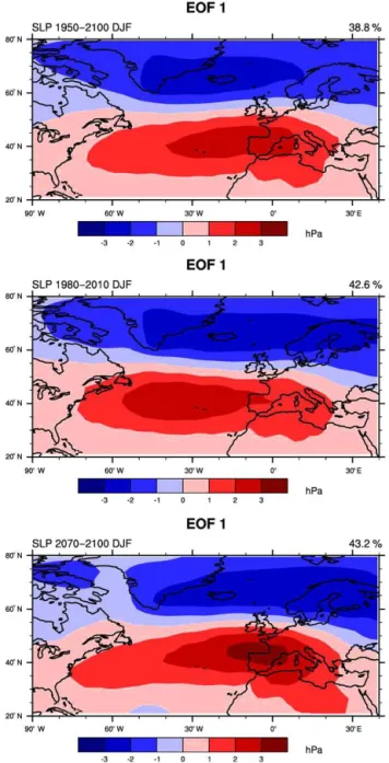
In order to define the spatial structure and temporal evo-lution of the NAO we use Empirical Orthogonal Function (EOF) analysis. We compute the eigenvectors of the cross-covariance matrix of the time variations of the SLP (Hurrell et al., 2003). By definition the eigenvectors are spatially and temporally mutually orthogonal and scale according to the amount of the total variance they explain; the leading EOF (EOF1) explains the largest percentage of the temporal vari-ance in the dataset. The NAO is identified by the EOF1 of the cross-covariance matrix computed from the SLP anoma-lies in the North Atlantic sector. The EOF1 spatial pattern is associated with a north–south pressure dipole with its cen-tres of action corresponding to the NAO poles with high-est SLP variability. Therefore, we compute the EOF1 from winter seasonal SLP anomalies in the North Atlantic sector (20–80◦N, 90◦W–40◦E) and we find that the long chem-istry coupled simulation (1950–2100) reproduces the NAO signal with the typical north–south dipole structure (Fig. 1, top). The EOF1 explains 38.8 % of the total variance, in ac-cordance with the results found in literature (e.g. Fischer et al., 2009; Ulbrich and Christoph, 1999). In order to detect the NAO differences between the past and the end of the 21st century, we define two 30-year-long periods referred to as “recent past” (1980–2010) and “future” (2070–2100). Fig-ure 1 (centre and bottom) shows the EOF1 analysis for the two distinct periods. A climatological timescale (30 years) for the two periods has been chosen to reduce the inter-decadal variability. Additionally, we have chosen various cli-matological timescales of 30 years during the past and future and we have computed the EOF1 in all periods, i.e. 1950– 1979, 1960–1989, 1970–1999, 1980–2009 in the past and 2040–2069, 2050–2079, 2060–2089, 2070–2099 in the fu-ture. The results (shown in Fig. S1 in the Supplement) exhibit differences between the two periods, past and future, but not
Figure 1.Leading empirical orthogonal function (EOF1) of the winter (DJF) mean sea-level pressure (SLP) anomalies in the North Atlantic sector (20–80◦N, 90◦W–40◦E) of the coupled simulation considering the full period 1950–2100 (top), recent past period: 1980–2010 (centre), and future period: 2070–2100 (bottom). The percentage at the top right of each figure quantifies the total vari-ance explained. The patterns are displayed in terms of amplitude (hPa), obtained by regressing the SLP anomalies on the principal component time series.
between any of the climatological timescales within each pe-riod. Thus, the changes observed for the past and future NAO patterns are not due to decadal variability but rather they are climate-induced.
Figure 2.Normalized principal component time series (PC1) of the leading empirical orthogonal function (EOF1) of the winter mean sea-level pressure (SLP) anomalies for the entire simulation period (1950–2100). The PC1 has been computed after removing the SLP climatology for the recent past (1980–2010).
NAO shift is in agreement with the results obtained by Ul-brich and Christoph (1999), Hu and Wu (2003) and Pausata et al. (2015) for a climate-change global-warming scenario.
The shift of the NAO centres of action has to be taken into account when examining the temporal evolution of the NAO pattern. The NAO station-based index, defined as the differ-ence in the normalized SLP between one northern station in Iceland and one southern station in the Azores, is fixed in space and is not able to capture the spatial variability of the NAO centres of action over seasonal (Hurrell et al., 2003) or (future) decadal (Ulbrich and Christoph, 1999) scales. Since our model projects a spatial shift of the NAO centres, we will be considering the principal component time series of the leading EOF of SLP (PC1) (Hurrell et al., 2003) as NAO temporal index. The normalized PC1 computed for the entire simulation (1950–2100) after subtracting the SLP climatol-ogy of 1980–2010 is shown in Fig. 2.
3.2 NAO changes
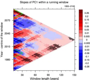
To investigate the NAO temporal variability and trends, we calculate, considering sliding windows, the linear regression coefficients with respect to time of the PC1 computed for the entire 150 year simulation (Fig. 2). In particular, we define windows of variable length between a minimum of 10 years and a maximum equal to 150 years sliding along the whole PC1 time series. We compute the linear slope (trend) for each window and assign the value to the win-dow central year (e.g. the regression coefficient of the PC1 series in the selected period 1980–1990, an 11 year win-dow, is assigned to the year 1985). Results in Fig. 3 show that no change in the projected future NAO variability is identified compared to the past when considering periods shorter than 30 years. For windows of length between 30 and 60 years, upward trends (centred in the 1980s and 2040s) in-terchange with downward trends (centred in the 2010s and 2060s). On longer window lengths we find that very weak non-statistically-significant NAO trends are prevalent. The
Figure 3.Linear regression coefficients of the PC1 based on cou-pled simulation data computed in sliding windows with variable length for the whole period 1950–2100. Plotted in thexaxis are the window lengths expressed in years, and in theyaxis the central year of the windows. The regression coefficient values are expressed in year−1(see colour legend). Points marked with black crosses in-dicate the 95 % level of significance. The green triangles inin-dicate the areas of the two periods, recent past and future.
slope of the overall trend computed for the entire PC1 is (2.99×10⁻³±0.95×10⁻³)[year−1], i.e. significant at 95 %.
In summary, our coupled EMAC–MPIOM model predicts a small significant positive trend for the NAO (for the 150 year horizon) in agreement with other studies that have used cou-pled models (e.g. Gillett et al., 2003; Hu and Wu, 2003; Stephenson et al., 2006). In the same plot (Fig. 3), we have marked two triangles in correspondence to the recent past and future periods, with the aim of stressing the NAO trend changes. In the lower triangle we distinguish two sharp pat-terns: an upward trend (red shading) which dominates be-tween 1980 and 1991 and a downward trend (blue shading) which dominates from 1992 onwards. Differently, in the up-per triangle we note that, at the end of the century, there is a clear prevalence of positive NAO trends.
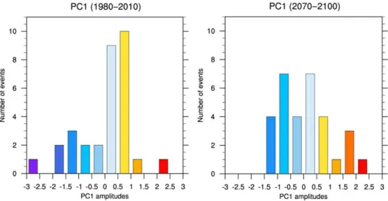
inter-Figure 4.NAO phase number distributions, computed in the recent past (left) and future (right) periods.
val[1;2.5]. Therefore, at the end of the century the number of negative NAO phases increases (15 in the future vs. 10 in the past) and, vice versa, the number of positive NAO phases decreases (16 in the future vs. 21 in the past). However, the “high NAO extreme events” (PC1>1.5) are more frequent in the future (4 in the future vs. 1 in the past), while the num-ber of “low NAO extreme events” (PC1<−1.5) decreases (0 in the future vs. 3 in the past), and such results are consistent with the future positive trend commented on before.
4 NAO effects on tracer transport in the future 4.1 Correlation and regression analysis
In order to investigate the NAO influence on tracer trans-port we compute the correlation (Fig. S2 in the Supplement) and the regression (Fig. 5) between the PC1 and tracer mix-ing ratio at the surface level. We consider passive tracers whose emissions and decay lifetime are constant (CO_25 and CO_50) in order to remove influences by chemical pro-duction and decomposition variability. In this way the anal-ysis gives information purely on the effect of tracer trans-port. We perform the correlation and regression considering the CO_25 tracer, which undergoes exponential decay with e-folding time equal to 25 days. A supplementary analysis is repeated for CO_50, with 50 days e-folding constant, to provide a constraint on the systematic uncertainty associated with the resident time of the tracer in the atmosphere and to show the robustness of our results. To identify the future changes in transport pathways related to the NAO, we per-form the analysis separately in the two periods, recent past and future.
By means of the correlation (Fig. S2) we determine where European and eastern USA CO-like tracers have a linear re-lationship with NAO. The higher the correlation (in
Figure 5.Regression of the winter seasonal CO_25 mixing ratio anomalies at surface level against the normalized PC1 computed for the recent past (left) and future (right) periods. The unit is mol mol−1and the points marked with a white cross indicate local significance at the 95 %.
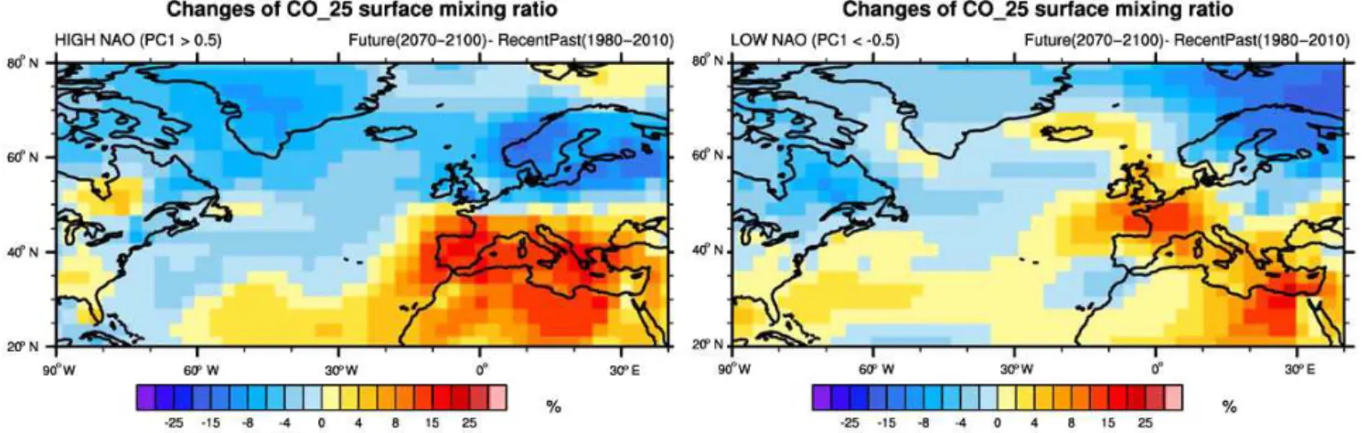
Figure 6.Differences between future (2070–2100) and recent past (1980–2010) temporal averages of CO_25 winter surface mixing ratio, both in the case of high NAO (PC1>0.5) (left) and low NAO (PC1<−0.5) (right). More precisely, plots show the results of[(CO_25futave−
CO_25pastave)/CO_25pastave] ×100, so the coloured bars indicate the percentages.
is also wider with respect to the past, and the magnitude of the negative correlation increases over north-eastern Eu-rope, southern Scandinavia, and the North Atlantic Ocean (between Great Britain and Iceland) with values in the range
−0.6 to−0.8. Again, the analysis considering CO_50 has produced similar results.
In order to better define the relationship between NAO and tracer transport, we regress the CO_25 mixing ratio against the normalized PC1 (Fig. 5). Analogously to the correlation, areas with positive values mean that positive/negative NAO phases drive a higher/lower stagnation of trace pollutants, while areas with negative values mean that positive/negative NAO phases drive a depletion/increment of such pollutants. However, in contrast to the correlation, the regression map shows how intense the effect of NAO on CO_25 concentra-tion could be. We observe that correlaconcentra-tion and regression pat-terns are very similar. The regression analysis shows that the flow over Europe transports tracers over the Arctic,
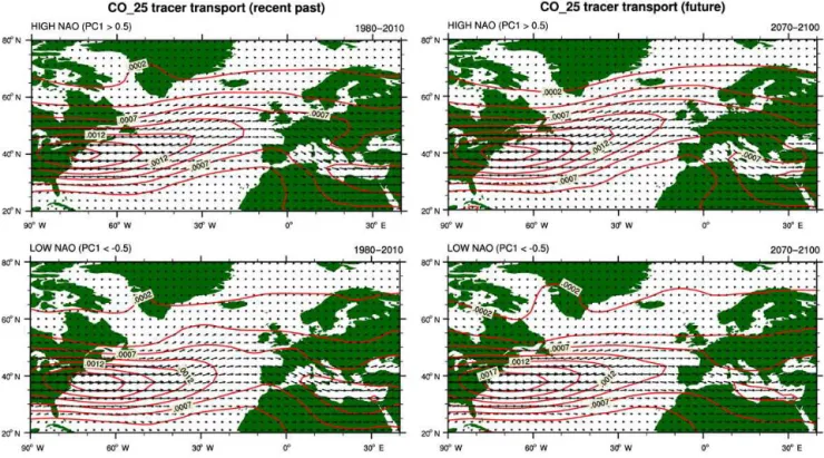
Figure 7.Temporal averages of vertically integrated CO_25 tracer transport vectors (molmolmkg·s) for winters with high NAO (PC1>0.5) (top) and low NAO (PC1<−0.5) (bottom), both in the recent past (left) and in the future (right).
to the Arctic and southward transport to Africa are further enhanced in the future. Such considerations are confirmed when studying the differences between future and recent past tracer concentration and transport (see next subsection).
Consequently, at the end of the century, the south-western Mediterranean and northern Africa will suffer from higher pollutant concentrations during positive NAO phases com-pared to the past, while a wider part of northern Europe will benefit from lower concentrations of long-range pollu-tants (associated with improved surface air quality) during the positive NAO phases with respect to the past. Similarly, the splitting over the American east coast will be enhanced as well, to a lesser degree. Nevertheless, we should note that this work is related only to the transport of CO-like tracers with constant lifetime and emissions, and thus it does not account for a possible (and probable) decrease of pollutant emissions both over Northern America and in Europe. More-over, we do not deal with the reduction of aerosol and aerosol precursors emissions, predicted by most of the representative concentration pathways (RCPs, Lamarque et al., 2011) over the Mediterranean, since we focus on trace gases rather than aerosols.
4.2 Tracer transport changes
Here, we further develop our analysis differentiating high and low NAO events, both in the recent past and in the future. We define “high NAO” and “low NAO” as (winter) periods
with PC1 higher than 0.5 and lower than−0.5, respectively. We obtain 12 high and 8 low NAO phases in the recent past and 9 high and 11 low NAO phases in the future. The aver-ages of the PC1 amplitudes (all computed over at least 8 val-ues) are equal to−1.38 in the recent past and−1.01 in the fu-ture considering the low NAO events and equal to 0.83 in the recent past and 1.24 in the future considering the high NAO events. Thus, we note that in the future the events categorized as high will have, on average, a higher PC1 amplitude than those in the recent past and, similarly, the future events cate-gorized as low will be less negative than those in the recent past. Therefore, we find that the number of low/high NAO events will increase/decrease in the future, while the mean PC1 amplitudes will increase in the future in both cases (low and high NAO).
(up to 15 %) and decrease over northern Scandinavia, the Arctic, and some areas of North America and the Atlantic Ocean (down to −10 %). Such variations are likely due to the more positive NAO events in the future. With this anal-ysis we corroborate the results of the previous subsection and, moreover, we estimate which concentration changes are associated with the different NAO phases. Nevertheless, we would like to stress that, while the correlation and regression analyses were performed over 30 years, here fewer years are considered (having to satisfy the conditions PC1<−0.5 or PC1>0.5).
Secondly, following the same definitions of high and low NAO, we compute the temporal averages ofQ(1). The main features of transport are in agreement with Hurrell (1995) and Christoudias et al. (2012): during positive NAO (Fig. 7, top) the axis of maximum transport has a southwest-to-northeast orientation across the Atlantic and extends farther to north-eastern Europe, while during negative NAO (Fig. 7, bottom) it is more longitudinally oriented. Comparing the recent past and future, we observe that during high NAO (Fig. 7, top) the east-northward transport of CO_25 is more pronounced in the future over the North Atlantic Ocean, from the northern American coast towards Ireland, while it gets weaker over southern Greenland, the Mediterranean and western Europe. During low NAO (Fig. 7, bottom), the eastward CO_25 transport over the North Atlantic Ocean extends farther eastwards in the future, while it decreases over the Mediterranean Sea and north-eastern Africa; in con-trast to the high NAO case, transport gets slightly stronger over southern Greenland in the future. For a more immediate comparison we have also computed the differences between the two periods and the results are shown in Fig. S5. The main future changes of CO_25 transport, which gets gener-ally stronger over the North Atlantic Ocean and weaker over the Mediterranean, confirm information retrieved from the correlation and regression analysis.
5 Conclusions
A free-running simulation performed by the coupled EMAC– MPIOM model has been analysed in order to study the influ-ence of the NAO on future pollutant transport and concen-tration changes. The simulation takes into account the GHG increment during the 21st century according to the ACCMIP (Lamarque et al., 2013) and RCP 6.0 scenario (Fujino et al., 2006) and uses a monthly aerosol climatology. The model is able to reproduce the SLP anomalies and the NAO signal (Christoudias et al., 2012), and the EOF analysis performed with the coupled simulation shows the typical dipole pattern which is identified as the NAO.
Similarly to other coupled GCMs, when considering the full modelled period in a global-warming scenario, our model projects (i) a northeastward shift of the NAO cen-tres of action (Ulbrich and Christoph, 1999; Hu and Wu,
2003; Pausata et al., 2015) and (ii) a very weak but signif-icant positive trend of the NAO (Hu and Wu, 2003; Gillett et al., 2003; Stephenson et al., 2006). This suggests that the an-thropogenic forcing has a non-null contribution in the NAO evolution. Moreover, in our model the NAO trends computed over periods shorter than 30 years will continue to oscillate between positive and negative values in the future. The anal-ysis of the NAO phase distribution reveals an increase of the negative NAO frequencies in the future although with much reduced amplitudes. On the contrary, positive NAO phases do decrease in frequency but increase in amplitude.
As far as the NAO impact on tracer transport is concerned, our results show that, in the recent past, NAO affected sur-face tracer concentrations with increased tracer concentra-tions over the Arctic, southern Mediterranean and northern Africa during positive NAO (similarly to the findings of Creilson et al., 2003; Eckhardt et al., 2003; Christoudias et al., 2012). Considering CO-like tracers with constant life-time and emissions, we find that, at the end of the century, the NAO effects on pollutants will be enhanced, i.e. tracer concentrations over those areas where they are depleted dur-ing positive NAO will reduce more, while they will increase over those areas to which they are transported. This means that tracers will be transported more efficiently towards those areas which already suffer from bad air-quality conditions during positive NAO, i.e. over the Arctic, southern Mediter-ranean and Africa.
Such conclusions are also confirmed by the computation of tracer mixing ratios and transport in the Atlantic sec-tor during high positive and low negative NAO phases. Fu-ture tracer concentrations during positive NAO will increase over central Europe, the southern Mediterranean and north-ern Africa, and reduce over northnorth-ern Europe and Greenland. Both the NAO amplitude changes and the NAO shift con-tribute to such concentration variations. For positive NAO, future tracer transport with respect to the past will get gener-ally stronger over the North Atlantic Ocean and weaker over the Mediterranean region, enhancing the depletion of pollu-tants from central-northern Europe and the stagnation over the southern Mediterranean and northern Africa. We remind that these results refer to constant emissions and idealized tracers (i.e. constant decay time).
6 Data availability
The Supplement related to this article is available online at doi:10.5194/acp-16-15581-2016-supplement.
Acknowledgements. The authors wish to extend their gratitude to the MESSy Consortium and the international IGAC/SPARC Chemistry–Climate Model Initiative (Eyring et al., 2013). The analysed simulations were carried out as part of the Earth System Chemistry integrated Modelling (ESCiMo) project at the German Climate Computing Centre (Deutsches Klimarechenzentrum, DKRZ). DKRZ and its scientific steering committee are gratefully acknowledged for providing the required computational resources.
The article processing charges for this open-access publication were covered by the Max Planck Society.
Edited by: P. Haynes
Reviewed by: two anonymous referees
References
Baldwin, M. P. and Dunkerton, T. J.: Stratospheric Harbingers of Anomalous Weather Regimes, Science, 294, 581–584, 2001. Christoudias, T., Pozzer, A., and Lelieveld, J.: Influence of the North
Atlantic Oscillation on air pollution transport, Atmos. Chem. Phys., 12, 869–877, doi:10.5194/acp-12-869-2012, 2012. Creilson, J. K., Fishman, J., and Wozniak, A. E.: Intercontinental
transport of tropospheric ozone: a study of its seasonal variabil-ity across the North Atlantic utilizing tropospheric ozone resid-uals and its relationship to the North Atlantic Oscillation, At-mos. Chem. Phys., 3, 2053–2066, doi:10.5194/acp-3-2053-2003, 2003.
Dietmüller, S., Jöckel, P., Tost, H., Kunze, M., Gellhorn, C., Brinkop, S., Frömming, C., Ponater, M., Steil, B., Lauer, A., and Hendricks, J.: A new radiation infrastructure for the Mod-ular Earth Submodel System (MESSy, based on version 2.51), Geosci. Model Dev., 9, 2209–2222, doi:10.5194/gmd-9-2209-2016, 2016.
Dorn, W., Dethloff, K., Rinke, A., and Roeckner, E.: Competition of NAO regime changes and increasing greenhouse gases and aerosols with respect to Arctic climate projections, Clim. Dy-nam., 21, 447–458, doi:10.1007/s00382-003-0344-2, 2003. Duncan, B. N. and Logan, J. A.: Model analysis of the factors
regulating the trends and variability of carbon monoxide be-tween 1988 and 1997, Atmos. Chem. Phys., 8, 7389–7403, doi:10.5194/acp-8-7389-2008, 2008
Eckhardt, S., Stohl, A., Beirle, S., Spichtinger, N., James, P., Forster, C., Junker, C., Wagner, T., Platt, U., and Jennings, S. G.: The North Atlantic Oscillation controls air pollution transport to the Arctic, Atmos. Chem. Phys., 3, 1769–1778, doi:10.5194/acp-3-1769-2003, 2003.
Eyring, V. and Lamarque, J.-F.: Global chemistry-climate modeling and evaluation, Eos, Transactions American Geophysical Union, 93, 539–539, doi:10.1029/2012EO510012, 2012.
Eyring, V., Lamarque, J. F., Hess, P., Arfeuille, F., Bowman, K., Chipperfield, M. P., Duncan, B., Fiore, A., Gettelman, A., Gior-getta, M. A., Granier, C., Hegglin, M., Kinnison, D., Kunze, M.,
Langematz, U., Luo, B., Martin, R., Matthes, K., Newman, P. A., Peter, T., Robock, A., Ryerson, T., Saiz-Lopez, A., Salawitch, R., Schultz, M., Shepherd, T. G., Shindell, D., Staehelin, J., Tegt-meier, S., Thomason, L., Tilmes, S., Vernier, J.-P., Waugh, D. W., and Young, P. J.: Overview of IGAC/SPARC Chemistry-Climate Model Initiative (CCMI) community simulations in support of upcoming ozone and climate assessments, SPARC Newsletter, 40, 48–66, 2013.
Fischer-Bruns, I., Banse, D. F., and Feichter, J.: Future impact of anthropogenic sulfate aerosol on North Atlantic climate, Clim. Dynam., 32, 511–524, doi:10.1007/s00382-008-0458-7, 2009. Fujino, J., Nair, R., Kainuma, M., Masui, T., and Matsuoka, Y.:
Multi-gas mitigation analysis on stabilization scenarios using aim global model, Energy J., 27, 343–354, 2006.
Fyfe, J. C., Boer, G. J., and Flato, G. M.: The Arctic and Antarctic Oscillations and their projected changes under global warming, Geophys. Res. Lett., 26, 1601–1604, 1999.
Gillett, N. P., Allen, M. R., McDonald, R. E., Senior, C. A., Shin-dell, D. T., and Schmidt, G. A.: How linear is the Arctic Oscilla-tion response to greenhouse gases?, J. Geophys. Res., 107, 4022, doi:10.1029/2001JD000589, 2002.
Gillett, N. P., Graf, H. F., and Osborn, T. J.: Climate change and the North Atlantic Oscilation, in: The North Atlantic Oscilla-tion: Climatic Significance and Environmental Impact, edited by: Hurrell, J. W., Kushnir, Y., Ottersen, G., and Visbeck, M. Geo-physical Monograph Series, 134, American GeoGeo-physical Union, Washington DC, 193–209, 2003.
Gillett, N. P. and Fyfe, J. C.: Annular mode changes in the CMIP5 simulations, Geophys. Res. Lett., 40, 1189–1193, doi:10.1002/grl.50249, 2013.
Hoerling, M. P., Hurrell, J. W., and Xu, T.: Tropical Origins for the Recent North Atlantic Climate Change, Science, 292, 90–92, doi:10.1126/science.1058582, 2001.
Hu, Z.-Z. and Wu, Z.: The intensification and shift of the annual North Atlantic Oscillation in a global warming scenario simula-tion, Tellus, 56A, 112–124, 2004.
Hurrell, J. W.: Decadal Trends in the North Atlantic Oscillation: Re-gional Temperatures and Precipitation, Science, 269, 676–679, 1995.
Hurrell, J. W., Kushnir, Y., and Visbeck, M.: The North Atlantic Oscillation, Science, 291, 603–602, 2001.
Hurrell, J. W., Kushnir, Y., Ottersen, G., and Visbeck, M.: An overview of the North Atlantic Oscillation, in: The North At-lantic Oscillation: Climatic Significance and Environmental Im-pact, edited by: Hurrell, J. W., Kushnir, Y., Ottersen, G., and Vis-beck, M., Geophysical Monograph Series, 134, American Geo-physical Union, Washington DC, 1–35, 2003.
Jöckel, P., Kerkweg, A., Pozzer, A., Sander, R., Tost, H., Riede, H., Baumgaertner, A., Gromov, S., and Kern, B.: Development cycle 2 of the Modular Earth Submodel System (MESSy2), Geosci. Model Dev., 3, 717–752, doi:10.5194/gmd-3-717-2010, 2010. Jöckel, P., Tost, H., Pozzer, A., Kunze, M., Kirner, O.,
Brenninkmei-jer, C. A. M., Brinkop, S., Cai, D. S., Dyroff, C., Eckstein, J., Frank, F., Garny, H., Gottschaldt, K.-D., Graf, P., Grewe, V., Kerkweg, A., Kern, B., Matthes, S., Mertens, M., Meul, S., Neu-maier, M., Nützel, M., Oberländer-Hayn, S., Ruhnke, R., Runde, T., Sander, R., Scharffe, D., and Zahn, A.: Earth System Chem-istry integrated Modelling (ESCiMo) with the Modular Earth Submodel System (MESSy) version 2.51, Geosci. Model Dev., 9, 1153–1200, doi:10.5194/gmd-9-1153-2016, 2016.
Kuzmina, S. I., Bengtsson, L., Johannessen, O. M., Drange, H., Bobylev, L. P., and Miles, M. W.: The North Atlantic Oscillation and greenhouse-gas forcing, Geophys. Res. Lett., 32, L04703, doi:10.1029/2004GL021064, 2005.
Lamarque, J.-F., Kyle, G. P., Meinshausen, M., Riahi, K., Smith, S. J., Vuuren, D. P., Conley, A. J., and Vitt, F.: Global and regional evolution of short-lived radiatively-active gases and aerosols in the Representative Concentration Pathways, Climatic Change, 109, 191–212, doi:10.1007/s10584-011-0155-0, 2011.
Lamarque, J.-F., Dentener, F., McConnell, J., Ro, C.-U., Shaw, M., Vet, R., Bergmann, D., Cameron-Smith, P., Dalsoren, S., Doherty, R., Faluvegi, G., Ghan, S. J., Josse, B., Lee, Y. H., MacKenzie, I. A., Plummer, D., Shindell, D. T., Skeie, R. B., Stevenson, D. S., Strode, S., Zeng, G., Curran, M., Dahl-Jensen, D., Das, S., Fritzsche, D., and Nolan, M.: Multi-model mean ni-trogen and sulfur deposition from the Atmospheric Chemistry and Climate Model Intercomparison Project (ACCMIP): evalu-ation of historical and projected future changes, Atmos. Chem. Phys., 13, 7997–8018, doi:10.5194/acp-13-7997-2013, 2013. Li, Q., Jacob, D. J., Bey, I., Palmer, P. I., Duncan, B. N., Field, B. D.,
Martin, R. V., Fiore, A. M., Yantosca, R. M., Parrish, D. D., Sim-monds, P. G., and Oltmans, S. J.: Transatlantic transport of pollu-tion and its effects on surface ozone in Europe and North Amer-ica, J. Geophys. Res., 107, 4166, doi:10.1029/2001JD001422, 2002.
Marsland, S., Haak, H., Jungclaus, J. H., Latif, M., and Röske, F.: The Max-Planck-Institute global ocean/sea ice model with orthogonal curvilinear coordinates, Ocean Modell., 5, 91–127, doi:10.1016/S1463-5003(02)00015-X, 2003.
Mehta, V. M., Suarez, M. J., Manganello, J. V., and Delworth, T. L.: Oceanic influence on the North Atlantic Oscillation and associ-ated Northern Hemisphere climate variations: 1959–1993, Geo-phys. Res. Lett., 27, 121–124, 2000.
Moulin, C., Lambert, C. E., Dulac, F., and Dayan, U.: Control of atmospheric export of dust from North Africa by the North At-lantic Oscillation, Nature, 387, 691–694, 1997.
NAO Index Data: provided by the Climate Analy-sis Section, NCAR, Boulder, USA, Hurrell, avail-able at: https://climatedataguide.ucar.edu/climate-data/ hurrell-north-atlantic-oscillation-nao-index-pc-based, (last access: 17 January 2016), 2003.
Osborn, T. J.,Briffa, K. R., Tett, S. F. B., Jones, P. D., and Trigo, R. M.: Evaluation of the North Atlantic Oscillation as simulated by a coupled climate model, Clim. Dynam., 15, 685–702, 1999. Pausata, F. S. R., Pozzoli, L., Vignati, E., and Dentener, F. J.: North
Atlantic Oscillation and tropospheric ozone variability in
Eu-rope: model analysis and measurements intercomparison, At-mos. Chem. Phys., 12, 6357–6376, doi:10.5194/acp-12-6357-2012, 2012.
Pausata, F. S. R., Pozzoli, L., Dingenen, R. V., Vignati, E., Cav-alli, F., and Dentener, F. J.: Impacts of changes in North At-lantic atmospheric circulation on particulate matter and hu-man health in Europe, J. Geophys. Res., 40, 4074–4080, doi:10.1002/grl.50720, 2013.
Pausata, F. S. R., Gaetani, M., Messori, G., Kloster, S., and Den-tener, F. J.: The role of aerosol in altering North Atlantic at-mospheric circulation in winter and its impact on air quality, Atmos. Chem. Phys., 15, 1725–1743, doi:10.5194/acp-15-1725-2015, 2015.
Pozzer, A., Jöckel, P., Tost, H., Sander, R., Ganzeveld, L., Kerk-weg, A., and Lelieveld, J.: Simulating organic species with the global atmospheric chemistry general circulation model ECHAM5/MESSy1: a comparison of model results with obser-vations, Atmos. Chem. Phys., 7, 2527–2550, doi:10.5194/acp-7-2527-2007, 2007.
Pozzer, A., Jöckel, P., Kern, B., and Haak, H.: The Atmosphere-Ocean General Circulation Model EMAC-MPIOM, Geosci. Model Dev., 4, 771–784, doi:10.5194/gmd-4-771-2011, 2011. Rauthe, M., Hense, A., and Paeth, H.: A model intercomparison
study of climate change-signals in extratropical circulation, Int. J. Climatol., 24, 643–662, doi:10.1002/joc.1025, 2004.
Rodwell, M. J., Rowell, D. P., and Folland, C. K.: Oceanic forc-ing of the wintertime North Atlantic Oscillation and European climate, Nature, 398, 320–321, 1999.
Roeckner, E., Brokopf, R., Esch, M., Giorgetta, M., Hagemann, S., Kornblueh, L., Manzini, E., Schlese, U., and Schulzweida, U.: Sensitivity of simulated climate to horizontal and vertical reso-lution in the ECHAM5 atmosphere model, J. Climate, 19, 3771– 3791, 2006.
Sander, R., Baumgaertner, A., Gromov, S., Harder, H., Jöckel, P., Kerkweg, A., Kubistin, D., Regelin, E., Riede, H., Sandu, A., Taraborrelli, D., Tost, H., and Xie, Z.-Q.: The atmospheric chem-istry box model CAABA/MECCA-3.0, Geosci. Model Dev., 4, 373–380, doi:10.5194/gmd-4-373-2011, 2011.
Saravanan, R.: Atmospheric Low-Frequency Variability and Its Relationship to Midlatitude SST Variability: Studies Using the NCAR Climate System Model, J. Climate, 11, 1386–1404, doi:10.1175/1520-0442(1998)011<1386:ALFVAI>2.0.CO;2, 1998.
Scaife, A. A. and Folland, C. K.: European Climate Extremes and the North Atlantic Oscillation, J. Climate, 21, 72–82, doi:10.1175/2007JCLI1631.1, 2007.
Shindell, D. T., Miller, R. L., Schmidt, G. A., and Pandolfo, L.: Sim-ulation of recent northern winter climate trends by greenhouse-gas forcing, Nature, 399, 452–455, 1999.
SPARC CCMVal: SPARC Report on the Evaluation of Chemistry-Climate Models, edited by: Eyring, V., Shepherd, T., and Waugh, D., SPARC Report No. 5, WCRP-30/2010, WMO/TD-No. 40, available at: http://www.sparc-climate.org/publications/ sparc-reports/ (last access: March 2016), 2010.
Thomas, M. A. and Devasthale, A.: Sensitivity of free tropospheric carbon monoxide to atmospheric weather states and their per-sistency: an observational assessment over the Nordic coun-tries, Atmos. Chem. Phys., 14, 11545–11555, doi:10.5194/acp-14-11545-2014, 2014.
Ulbrich, U. and Christoph, M.: A shift of the NAO and increas-ing storm track activity over Europe due to anthropogenic green-house gas forcing, Clim. Dynam., 15, 551–559, 1999.
Visbeck, M. H., Hurrell, J. W., Polvani, L., and Cullen, H. M.: The North Atlantic Oscillation: past, present, and future, P. Natl. Acad. Sci. USA, 98, 12876–12877, doi:10.1073/pnas.231391598, 2001.
Walker, G. T. and Bliss, E. W.: World Weather, V. Mem. Roy. Me-teorol. Soc., 4, 53–83, 1932.
Woollings, T., Franzke, C., Hodson, D. L. R., Dong, B., Barnes, E. A., Raible, C. C., and Pinto, J. G.: Contrasting interannual and multidecadal NAO variability, Clim. Dynam., 45, 539–556, doi:10.1007/s00382-014-2237-y, 2015.