ISSN 0101-8205 www.scielo.br/cam
The uncertainty effects of deformation bands
on fluid flow
MICHAEL PRESHO1, VICTOR GINTING1 and SHAOCHANG WO2
1Department of Mathematics, University of Wyoming,
1000 East University Avenue, Laramie, WY 82071
2Enhanced Oil Recovery Institute, University of Wyoming,
1000 East University Avenue, Laramie, WY 82071
E-mails: [email protected] / [email protected] / [email protected]
Abstract. Reservoir fractures and deformation bands are capable of affecting fluid flow and
storage in a variety of ways. In terms of flow effects, we typically encounter an unchanged
or increased permeability when considering flow parallel to a fracture, whereas we expect a
noticeably reduced permeability when considering flow across (perpendicular to) a deformation
band. For this paper, we refine our efforts and focus on the effects of deformation bands on
multi-component porous medium flow. The main assumption is that the width of the band is a
random (uncertain) variable that follows a certain statistical distribution from which a number of
realizations can be generated. Monte Carlo simulations can then be performed to obtain statistical
representations of the transport quantity in relation to the nature of uncertainty. As analytical
expressions are available for this quantity of interest, we are able to compare them with the
Monte Carlo results. Furthermore, we derive a stochastic perturbation model as an alternative
to Monte Carlo simulations. Finally, a set of numerical examples is presented to illustrate the
performance of these approaches.
Mathematical subject classification: 65C20.
Key words: deformation band, pressure equation, saturation equation, Monte Carlo,
uncer-tainty, stochastic perturbation expansion.
1 Introduction
Deformation bands typically represent sections of porous media with signifi-cantly reduced permeability and porosity resulting from cementation [8]. The decreased permeability inhibits fluid flow, contributes to a higher pressure drop, and as a result, deformation bands can play a role in reservoir fluid flow [8]. The study of deformation bands extends to various areas of academia and in-dustry, and in this paper we address the topic within a mathematical framework [1, 8, 17, 18]. For our particular petroleum industry application, we are inter-ested in quantifying the effects of deformation bands on oil production. This can be done by assigning uncertainty to various parameters that describe a band. The effects of deformation band permeability, orientation, and width (aperture) have been studied in a non-mathematical framework [8]. As a result, we as-sume that the above parameters can represent random variable candidates in the initial problem formulation.
In this study, we treat the width of a deformation band as the random variable of interest. This is a natural choice since variation in the width of a band is often guaranteed in a subsurface reservoir [8]. In other words, knowledge that deformation bands exist in a reservoir does not offer much information about the width(s) of the bands. We also point out that wider bands progressively inhibit flow (due to the reduced permeability), and thus the width is a pa-rameter that can most directly affect oil production in a porous medium [8]. With width as the random variable, we make deterministic assumptions on the permeability and location of a vertically oriented deformation band in an ideal-ized porous medium. These initial assumptions offer a foundation in describing the physical model. The multi-component flow under consideration is mod-eled by a hyperbolic partial differential equation coupled with Darcy’s Law [2, 3, 4, 16]. Within this setting, the velocity and saturation become functions of a random variable due to their dependence on the deformation band’s width. In turn, the oil production is also random.
so-lutions we can use the probability density function to compute exact statistical mean values. These exact values give a benchmark of comparison with numeri-cal methods that assess the effects of uncertainty. One such method is the Monte Carlo method. This method involves generating a number of realizations of a random variable and then averaging over the realizations to obtain effective solu-tions [9]. In the scope of our problem, we choose a probability density function, generate a number of realizations for the width of a deformation band, and com-pute the statistical mean production curves. Monte Carlo is a widely used tool and much of today’s computing power is devoted to calculating Monte Carlo solutions [6]. However, one main disadvantage is that Monte Carlo is a very expensive method to implement, particularly if a large number of realizations is required. It is this disadvantage that leads us to explore more efficient methods of computing expectations.
In order to address the costly aspect of Monte Carlo, we introduce a stochastic perturbation model. The derivation of the model hinges on the assumption that the saturation and velocity can be expressed as first order stochastic perturbations (see, for example [13, 14, 19]). Using this assumption we can then reintroduce the variables into the original equations to obtain a governing equation for the saturation statistical mean. In deriving the model we make two main assump-tions. First, we assume that a first spatial derivative does not change significantly along a characteristic. Second, we assume that any third order stochastic terms can be neglected. The resulting model is, in general, more efficient than Monte Carlo and offers solutions that very closely match Monte Carlo for low devi-ations. We note that this approach has been previously introduced by Glimm and Sharp, and Zhang [11, 21] (see also [20]). Within the context of upscal-ing in heterogeneous flow a similar approach has been used in [5, 7, 10, 15]. However, for higher deviations we encounter solutions that stray slightly from Monte Carlo. This is due to the fact that we neglect a third order stochastic term in the model derivation. We classify the latter results as a limitation of the model, however, we remark that the model still performs reasonably well regardless of some discrepancies found for higher deviations.
de-formation band is random we solve the respective set of equations analytically. By doing so, we eliminate any errors that may arise from numerical approxima-tion and focus solely on the effects of uncertainty. In §3 we use the analytical solutions to calculate the Monte Carlo production curves using both Uniform and Gaussian distributions [12]. As the exact statistical mean is available in these cases, we can make a comparison with the Monte Carlo results. In §4 we derive a stochastic perturbation model which hinges on expressing the saturation and velocity as first order stochastic perturbations. In §5 we solve the model numerically and compare the results with the Monte Carlo solutions from §3. In addition, we perform a probability density function comparison. Finally, we offer some concluding remarks in §6.
2 Model equations
In this section we begin by introducing the hyperbolic saturation equation that models a general two-component system. Letting S denote the saturation of a displacing fluid, we consider
∂S
∂t +v(t)
∂S
∂x =0
S(x,0)=0
S(0,t)=1,
(1)
where x ∈ [0,L], t ∈ [0,∞), and v(t) = − k
μ(S)
d p
d x is the flux obtained
through the pressure equation
− d d x
k(x) μ(S)
d p d x
=0,
p(0)= p0,
p(L)= pL,
(2)
which is coupled to (1) through the viscosity
μ(S)= μo
[M14S+(1−S)]4
. (3)
The parameter M = μo
μd
is the viscosity ratio, μodenotes the viscosity of the
two-component flow, we assume that M < 1. This models a polymer flood situation where the polymer (displacing fluid) component is more viscous than
the oil component. A single phase flow is a special case in which, M = 1,
i.e., there is only one fluid present.
Within this framework, we useβ to denote the random width of the deforma-tion band and assume a piecewise constant permeability structure
k(x;β)=
k1ifx ∈ [0,L−2β)
k2ifx ∈ [L−2β, L+2β] k3ifx ∈(L+2β,L].
(4)
See Figure 1. We are particularly interested in the situation wherek1=k3=kf
andk2 =kb <kf. Herekf represents the field permeability, andkbrepresents
the permeability within a deformation band.
0 20 40 60 80 100
0 100 200 300 400 500 600 700 800
Permeability Structure
x
k
k1 − field
k 2 − d.b. k
3 − field
Figure 1 – General permeability structure.
In solving (1) analytically we ultimately want to derive an expression for the location of the saturation front. We denote this location byξ(t;β). Upon successfully finding this quantity, the saturation solution is
S(x,t;β)=
(
1 if x < ξ(t;β)
0 if x > ξ(t;β). (5)
Furthermore, we eventually want to analyze the uncertainty effects of the pro-duction curveF(t;β)defined as
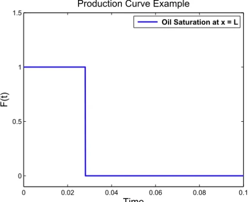
F(t;β)=1−S(L,t;β). (6) The production curve essentially shows us the saturation of oil at the right bound-ary,L, of our interval. See Figure 2 for an example of a production curve plotted against time.
0 0.02 0.04 0.06 0.08 0.1
0 0.5 1 1.5
Production Curve Example
Time
F
(t
)
Oil Saturation at x = L
Figure 2 – Production curve for a given value ofv.
Generally speaking, to solve forξ(t;β), we must first derive the flux. Then we set dξ
dt =v(ξ ). From here we arrive at an equation forξ which can easily
L L+β
2 L−β
2 0
µ(1)
ξ1
k3
k2 µ(0)
k1
L L+β
2 L−β
2 0
µ(1)
k3
k2 µ(0)
k1
ξ2
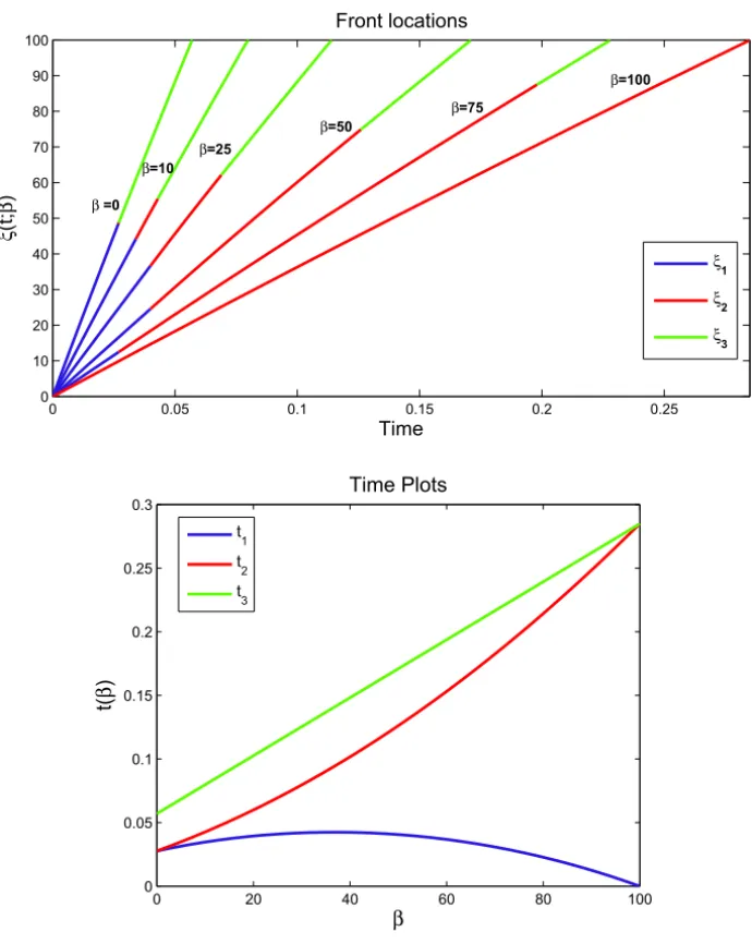
Figure 3 – Front locationsξ1andξ2advancing in time. ξ1describes the movement of
the front to the left of the deformation band, andξ2describes the movement of the front
within the deformation band.
cases for the flux and front location. See Figure 3. In particular, we have three separate flux values
v(ξ )=v(ξi) for ξi ∈(xi−1,xi), i =1,2,3, (7)
wherex0=0, x1= L−2β, x2= L+2β, and x3=L depending on where ξ lies in the spatial interval. In addition, when the porous medium is fully saturated,
v=vs for ξ >x3, (8)
i.e., the front has passed the right boundary. Treating each case separately, using (2) and (4), and ensuring continuity atξ we obtain
v(ξi(t;β))=
1p
miξi +niβ+qi
for ξi ∈(xi−1,xi), i=1,2,3, (9)
where 1p= p0−pL, and mi, ni, and qi are deterministic values depending on the parameterskf,kb,L, andM. As a representative example,
m1= μ(1)−μ(0) kf
, n1= μ(0)
kb −
μ(0)
kf
, and q1= Lμ(0)
kf
. (10)
Furthermore,
vs(β)=
1p
nsβ+qs for ξ >x3 (11)
is the fully saturated flux value, where ns andqs are similarly deterministic. Using (9) we can now setdξ
differential equation for each case. Treating each case separately and ensuring continuity we arrive at a quadratic equation forξi fori = 1,2,3. In addition,
we can solve for theβ dependent times when the front values shift:
t1(β)=t :ξ1(t;β)=ξ2(t;β)=x1 , t2(β)=t :ξ2(t;β)=ξ3(t;β)=x2 , and t3(β)=t :ξ3(t;β)=x3 .
(12)
See Figure 4 for a plot of the front locations and time values. Of particular interest,ξ3takes the form
ξ3(t;β)=
−(n3β+q3)+p(n3β+q3)2+2m3∙σ (m3,n3,q3,t;β)
m3 , (13)
whereσ is readily accessible.
Then (13) is appropriately used to evaluate S(L,t) from (1). We remark that we are considering a model that yields a random fluid velocity. In turn, (1) gives a random, analytical saturation solution. With this solution we can now implement the Monte Carlo method and compute statistical mean values of production.
3 Monte Carlo results
The Monte Carlo simulation is implemented for two-component and single phase flows. We generate N =10,000 positive realizations ofβ from Gaussian and Uniform distribution, with fixedhβi = 10 and various standard deviations,σβ. For each realization βi we compute ξ3i(t;β), i = 1, . . . ,N from (13), and
subsequently a production curve Fi(t)from (1). We then average the values at each time level and plot the resulting statistical mean production curve given by
hF(t)iMC =
1
N N
X
i=1
Fi(t). (14)
The deterministic data arekf =500,kb=100,L =100, p0 =1000, pL =0,
μo =2.7, andμd =3 (for two-component flow) andμo =μd =1 (for single
0 0.05 0.1 0.15 0.2 0.25 0
10 20 30 40 50 60 70 80 90 100
Front locations
Time
ξ
(t
;
β
)
ξ1
ξ2
ξ3 β =0
β=25
β=50
β=75
β=10
β=100
0 20 40 60 80 100
0 0.05 0.1 0.15 0.2 0.25 0.3
Time Plots
β
t(
β
)
t
1
t
2
t
3
Figure 4 – Front locations and times.
For the problem we consider, convergence of the Monte Carlo simulation can be accessed by way of comparison to the exact production curve statistical mean expressed as
hF(t)i =
Z L
0
1−S(L,t;β)
where fβ(β)is the respective probability density function of the Gaussian or Uniform distribution [12]. This comparison is presented in Figure 5, showing
for single phase flow and two-component flow. We choseσβ = 10 as a
mid-dle ground for comparison. The two results are indistinguishable from each
other which indicates the convergence of Monte Carlo for the N = 10,000
realizations.
0 0.01 0.02 0.03 0.04 0.05 0.06 0.07 0.08
0 0.5 1 1.5
Single Phase, Gaussian Distribution
Time
〈
F
(t
)
〉
MC − 10,000 Real. Exact
0 0.01 0.02 0.03 0.04 0.05 0.06 0.07 0.08
0 0.5 1 1.5
Single Phase, Uniform Distribution
Time
〈
F
(t
)
〉
MC − 10,000 Real. Exact
0 0.05 0.1 0.15 0.2
0 0.5 1 1.5
Two−Component, Gaussian Distribution
Time
〈
F
(t
)
〉
MC − 10,000 Real. Exact
0 0.05 0.1 0.15 0.2
0 0.5 1 1.5
Two−Component, Uniform Distribution
Time
〈
F
(t
)
〉
MC − 10,000 Real. Exact
Figure 5 – Comparison of Monte Carlo and Exact Statistical Mean of Production Curve withσβ =10: Single Phase (top), Two-Component (bottom).
0 0.01 0.02 0.03 0.04 0.05 0.06 0.07 0.08 0
0.5 1 1.5
Single Phase, Gaussian Distribution
Time 〈 F (t ) 〉 σ β = 0 σβ = 2 σβ = 5 σ
β = 10 σβ = 15
0 0.01 0.02 0.03 0.04 0.05 0.06 0.07 0.08
0 0.5 1 1.5
Single Phase, Uniform Distribution
Time 〈 F (t ) 〉 σ β = 0 σβ = 2 σβ = 3 σ
β = 5 σβ = 10
0 0.05 0.1 0.15 0.2
0 0.5 1 1.5
Two−Component, Gaussian Distribution
Time 〈 F (t ) 〉
σβ = 0 σ
β = 2 σβ = 5 σ
β = 10 σβ = 15
0 0.05 0.1 0.15 0.2
0 0.5 1 1.5
Two−Component, Uniform Distribution
Time 〈 F (t ) 〉
σβ = 0 σ
β = 2 σβ = 3 σ
β = 5 σβ = 10
Figure 6 – Monte Carlo Statistical Mean Production Curves for various σβ: Single Phase (top), Two-Component (bottom).
the left of breakthrough time for higher deviations. We generally expect earlier breakthrough when assuming more uncertainty. In the case of the realizations from the Uniform distribution, we see solutions that sharply deviate from the deterministic solution. Higher deviations lead to predictably increased variation after breakthrough and earlier breakthrough times. In general, we see similar pattern for higher deviations only with sharper curves.
4 Stochastic perturbation expansion
Thus far we have computed statistical mean of the production curves using Monte Carlo simulation and gave comparison with their exact counterparts. We reiterate the fact that Monte Carlo is, in general, an expensive computational approach. This is particularly the case when a large number of realizations is desired. To address this issue we now consider a separate, less costly method of comput-ing statistical values in relation to our problems. In particular, we will derive an equation governing the statistical mean of the saturation Susing the notion of Stochastic perturbation expansion. Recall the fact thatv(t)and S(x,t)are random functions due to their dependence onβ. To simplify notations, we will now use
hS(x,t)i = ˉS(x,t) and hv(t)i = ˉv(t).
Stochastic perturbation assumption allows us to express these variables as
S(x,t)= ˉS(x,t)+S′(x,t) and v(t)= ˉv(t)+v′(t), (15) where S′(x,t) andv′(t)are stochastic fluctuation terms. Substitution of (15) into (1) and appropriately rearranging the resulting equation yield
∂Sˉ
∂t + ˉv(t)
∂Sˉ
∂x
+
∂S′
∂t + ˉv(t)
∂S′
∂x
= −v′(t)
∂Sˉ
∂x +
∂S′
∂x
. (16)
By taking the expected value of (16) and usingS′ =v′ =0, we get
∂Sˉ
∂t + ˉv(t)
∂Sˉ
∂x +v
′(t)∂S ′
∂x =0. (17)
Here we have obtained a governing equation for statistical mean of the saturation. Our next task is to model the second order effectv′(t)S′
x. To accomplish this
we now work on the characteristicsv(ˉ t) = d x/dt. Using the notion of a total derivative, (16) becomes
dSˉ dt +
d S′ dt +v
′(t)∂Sˉ
∂x = −v
′(t)∂S ′
∂x . (18)
Integration along the characteristic, with the assumption thatSxˉ does not signif-icantly change along the characteristics yield
ˉ
S(x(t),t)+S′(x(t),t)+∂ ˉ S
∂x
Z t
0
v′(τ )dτ = −
Z t
0
v′(τ )∂S
′
Multiplying byv′(t), taking expectation, and neglecting the higher order stochas-tic term give
v′(t)S′(x(t),t)≈ −v′(t)
Z t
0
v′(τ )dτ∂Sˉ
∂x,
and therefore,
v′(t)∂S ′
∂x ≈ −v
′(t)
Z t
0
v′(τ )dτ∂
2Sˉ
∂x2. (19)
Substitution of (19) into (17) yields
∂Sˉ
∂t + ˉv(t)
∂Sˉ
∂x −α(t)
∂2Sˉ
∂x2 =0, (20)
where
α(t)=v′(t)
Z t
0
v′(τ )dτ . (21)
For single phase flow, the flux is independent of time and thusα(t) = σv2∙t. The above differential equation is completed by imposing a natural boundary condition
∂Sˉ
∂x(L,t)=0,
in addition to the existing initial and boundary conditions from the original problem.
We note that more general equations were derived in [11] and [21] for single phase flow. In particular, Glimm and Sharp (see [11]) and Zhang (see [21]) ob-tained related results in the context of a multi-length-scale, random permeability field. For two phase flow, we refer the reader to [20].
5 Comparison of approaches
This section is devoted for comparison between the Monte Carlo simulation and the Stochastic Perturbation Expansion described in the previous section. To solve (20) we use a Backward Euler, centered finite difference scheme where
∂S
∂t(xi,tn)≈
Sin−Sin−1
1t ,
∂S
∂x(xi,tn)≈ Sn
i+1−Sin−1
21x and
∂2S
∂x2(xi,tn)≈ Sn
i+1−2Sin+Sin−1
The equation is solved on a very fine grid and very small time steps in order to minimize any sources of error from numerical discretization. In particular, we want to focus solely on the effects of uncertainty. We point out that the first step in solving the model is the computation ofv(ˉ t)andα(t).
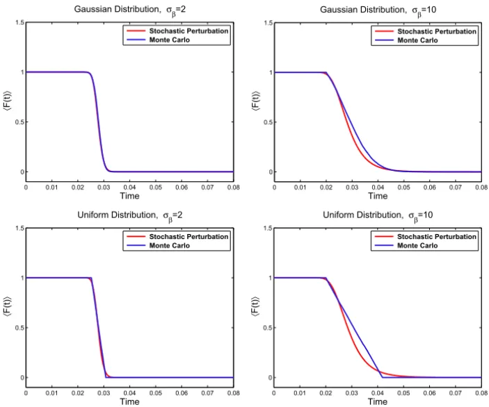
Comparison for single phase flow is presented in Figure 7. We use a relatively low deviation,σβ =2, and a relatively high deviation,σβ =10. In addition, the Gaussian and Uniform distributions are used for modeling the random behavior ofβ.
0 0.01 0.02 0.03 0.04 0.05 0.06 0.07 0.08
0 0.5 1 1.5
Gaussian Distribution, σ
β=2
Time
〈
F
(t
)
〉
Stochastic Perturbation Monte Carlo
0 0.01 0.02 0.03 0.04 0.05 0.06 0.07 0.08
0 0.5 1 1.5
Gaussian Distribution, σβ=10
Time
〈
F
(t
)
〉
Stochastic Perturbation Monte Carlo
0 0.01 0.02 0.03 0.04 0.05 0.06 0.07 0.08
0 0.5 1 1.5
Uniform Distribution, σβ=2
Time
〈
F
(t
)
〉
Stochastic Perturbation Monte Carlo
0 0.01 0.02 0.03 0.04 0.05 0.06 0.07 0.08
0 0.5 1 1.5
Uniform Distribution, σβ=10
Time
〈
F
(t
)
〉
Stochastic Perturbation Monte Carlo
Figure 7 – Comparison of Stochastic Perturbation to Monte Carlo for Single Phase Flow.
is reasonable. Forσβ = 10 we see an accurate portrayal of the breakthrough time, yet there is a noticable smoothing at the drop. This is expected as the model is parabolic. We recall that in §4 we also made the assumption that a third order stochastic term could be neglected. Forσβ =10 we simply see the natural breakdown of this assumption.
We now shift our attention to the Uniform case. In this case, we encounter similar behavior of the model solutions (with respect to the Gaussian model solutions). The main difference is that we see pronounced smoothing as com-pared to the Uniform Monte Carlo curves. Again, this is expected since the model is parabolic, whereas the Monte Carlo curves are inherently sharper in the Uniform case. Similarly, we see an accurate portrayal of breakthrough time even for a higher deviation, yet a discrepancy after that.
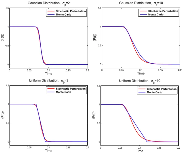
The results for the model applied to the two-component case are shown in Figure 8. We use a relatively low deviation, σβ = 2, and a relatively high deviation,σβ =10 for the Gaussian disbribution, while for the Uniform distri-bution we useσβ =3 andσβ =10.
The stochastic perturbation model agrees with the Monte Carlo solutions for a low deviation, while similar behavior as in single phase flow occurs for a higher deviation. We encounter similar behavior of the model solutions for the Uniform distribution (see Fig. 8). The main difference is that we see pronounced smoothing as compared to the Monte Carlo curves. Again, this is not a surprise since the model is parabolic, whereas the Monte Carlo curves are inherently sharper in the Uniform case.
Next we offer a comparison between the Gaussian and Uniform distribu-tion results. At this point, we have treated each case separately in comput-ing the Monte Carlo and numerical solutions. However, we think it is bene-ficial to offer a side by side comparison. For these comparisons we only con-sider the two-component case, although the same conclusions hold in the single phase case.
0 0.05 0.1 0.15 0.2 0
0.5 1 1.5
Gaussian Distribution, σβ=2
Time 〈 F (t ) 〉 Stochastic Perturbation Monte Carlo
0 0.05 0.1 0.15 0.2
0 0.5 1 1.5
Gaussian Distribution, σβ=10
Time 〈 F (t ) 〉 Stochastic Perturbation Monte Carlo
0 0.05 0.1 0.15 0.2
0 0.5 1 1.5
Uniform Distribution, σβ=3
Time 〈 F (t ) 〉 Stochastic Perturbation Monte Carlo
0 0.05 0.1 0.15 0.2
0 0.5 1 1.5
Uniform Distribution, σβ=10
Time 〈 F (t ) 〉 Stochastic Perturbation Monte Carlo
Figure 8 – Comparison of Stochastic Perturbation to Monte Carlo for Two-Compo-nent Flow.
0 0.05 0.1 0.15 0.2
0 0.5 1 1.5 Monte Carlo Time 〈 F (t ) 〉 Uniform Gaussian
0 0.05 0.1 0.15 0.2
0 0.5 1 1.5 Stochastic Perturbation Time 〈 F (t ) 〉 Uniform Gaussian
We also compare the solutions of (20) as solved with both the Gaussian and Uniform distributions (right side of Figure 9). Interestingly, the numerical so-lutions are quite similar to one another. This indicates that the model is not very sensitive to the probability density function we use to calculate the required coefficients. The curves are identical near the breakthrough time, and differ ever so slightly after breakthrough.
6 Conclusion
In this paper we introduce a stochastic perturbation model to quantify the effect of uncertainty of the deformation band width to oil production. By expressing our saturation and velocity quantities in terms of first order stochastic pertur-bations we are able to obtain from the original equations a parabolic equation modeling the statistical mean values of saturation. For low deviations we en-counter solutions that almost exactly coincide with the Monte Carlo results. For higher deviations we see discrepancies with the Monte Carlo results that can be attributed to the assumptions in the model derivation. We ultimately obtain a more efficient method for computing expected saturation values and we verify the accuracy by first computing Monte Carlo production curves (with a variety of deviations) for the single phase and two-component saturation equations. In ad-dition, we conclude that the model is not sensitive with respect to the probability density functions of interest (Gaussian or Uniform).
REFERENCES
[1] A. Aydin, Small Faults Formed as Deformation Bands in Sandstone. Pageoph,116(1978), 913–930.
[2] J. Bear,Dynamics of Fluids in Porous Media. Courier Dover Publications (1988).
[3] L.P. Dake,Fundamentals of Reservoir Engineering. Elsevier (1978).
[4] H. Darcy,Les Fontaines Publiques de la Ville de Dijon. Dalmont, Paris (1856).
[5] Y.R. Efendiev, L.J. Durlofsky and S.H. Lee, Modeling of subgrid effects in coarse scale simulations of transport in heterogeneous porous media. Water Resour. Res.,36(2000), 2031–2041.
[7] R. Ewing, Y. Efendiev, V. Ginting and H. Wang, Upscaling of Transport Equations for Multiphase and Multicomponent Flows. Lect. Notes Comput. Sc. Eng.,60(2008), 193–200.
[8] H. Fossen and A. Bale, Deformation bands and their influence on fluid flow. AAPG Bull.,
91(12) (2007), 1685–1700.
[9] J.E. Gentle,Random Number Generation and Monte Carlo Methods. Springer Verlag, (2003).
[10] V. Ginting, R. Ewing, Y. Efendiev and R. Lazarov, Upscaled modeling in multiphase flow applications. Comput. Appl. Math.,23(2-3) (2004), 213–233.
[11] J. Glimm and D. Sharp, A Random Field Model for Anomalous Diffusion in Heteroge-neous Porous Media. J. Stat. Phys.,62(1-2) (1991), 415–424.
[12] W.L. Hays,Statistics. Wadsworth Publishing Company (1994).
[13] M. Kami´nski, Application of the generalized perturbation-based stochastic boundary ele-ment method to the elastostatics. Eng. Anal. Bound. Elem.,31(6) (2007), 514–527.
[14] M. Kami´nski, Generalized Stochastic Perturbation Technique in Engineering Computa-tions. J. Eng. Appl. Sci.,3(3) (2008), 246–260.
[15] P. Langlo and M.S. Espedal, Macrodispersion for two-phase, immisible flow in porous media. Adv. Water Resour.,17(1994), 297–316.
[16] P.D. Lax, Hyperbolic Systems of Conservation Laws and the Mathematical Theory of Shock Waves. SIAM, Philadelphia (1973).
[17] T. Manzocchi, P.S. Ringrose and J.R. Underhill, Flow through fault systems in high-porosity sandstones. Struct. Geol. Reservoir Characterization,127(1998), 65–82.
[18] K.R. Sternlof, M. Karimi-Fard, D.D. Pollard and L.J. Durlofsky,Flow and transport effects of compaction bands in sandstone at scales relevant to aquifer and reservoir management. Water Resour. Res.,42(2006), W07425.
[19] D. Tartakovsky and A. Guadagnini, Prior mapping for nonlinear flows in random environ-ments. Phys. Rev. E.,64(2001), 03530(R).
[20] D. Zhang, Stochastic Methods for Flow in Porous Media. Coping With Uncertainties. Academic Press, San Diego, CA (2002).