ISSN 0101-8205 www.scielo.br/cam
Recurrence relations between moments of order
statistics from doubly truncated Makeham distribution
A.W. ABOUTAHOUN and N.M. AL-OTAIBI
Department of Mathematics, King Saud University, Riyadh, Kingdom of Saudi Arabia E-mail: [email protected]
Abstract. In this paper, we present recurrence relations between the single and the product
moments for order statistics from doubly truncated Makeham distribution. Characterizations for the Makeham distribution are studied.
Mathematical subject classification: 62G30, 65C60.
Key words: moments of order statistics, Makeham distribution, doubly truncated
distribu-tion, recurrence relations.
1 Introduction
Many researchers have studies the moments of order statistics of several distri-butions. A number of recurrence relalations satisfied by these moments of order statistics are available in literature. Balakrishnan and Malik [2] derived some identities involving the density functions of order statistics. These identities are useful in checking the computation of the moments of order statistics. Bala-krishnan and Malik [3] established some recurrence relations of order statistics from the liear-expoential distribution. Balakrishnan et al. [4] reviewed several recurrence relations and identities for the single and product moments of order statistics from some specific distributions. Mohie El-Din et al. [9, 10] presented recurrence relations for the single and product moments of order statistics from the doubly truncated parabolic and skewed distribution and linear-exponential distribution. Hendi et al. [1] developed recurrence relations for the single and
product moments of order statistics from doubly truncated Gompertz distribu-tion. Khan et al. [7] established general result about recurrence relations between product moments of order statistics. They used that result to get the recur-rence relations between product moments of some doubly truncated distribu-tions (Weibull, expoential, Pareto, power function, and Cauchy). Several recur-rence relations satisfied by these moments of order statistics are also available in Khan and Khan [5], [6].
The probability density function (pdf) of the Makeham distribution is given by
fX(x)= 1+θ 1−e−x
e−x−θ(x+e−x−1), x ≥0, θ ≥0 The doubly truncated pdf of continuous rv is given by
f(x)= fX(x)
P−Q =
1
P−Q 1+θ 1−e
−x
e−x−θ(x+e−x−1), Q1≤x ≤ P1
(1.1)
where
1−P =e−P1−θ(P1+e−P1−1) and 1−Q=e−Q1−θ(Q1+e
−Q1−1)
The cumulative distribution functionc.d.f. is given by 1−F(x)= f(x)
1+θ (1−e−x)−P2 (1.2) where
P2= 1−P
P−Q
Let X be a continuous random variable having ac.d.f. (1.2)andp.d.f.. Let
X1,X2, . . . ,Xn be a random sample of sizen from the Makeham distribution and X1:n ≤ X2:n ≤ ∙ ∙ ∙ ≤ Xn:n be the corresponding order statistics obtained from the doubly truncated Makeham distribution(1.1), then
fr:n(x)=Cr:n[F(x)]r−1[1−F(x)]n−r f (x) (1.3) where
Cr:n =
n!
The expected value of any measurable functionh(x)can be obtained as fol-lows:
αr:n =E[h(Xr:n)]=
Cr:n
Z P1 Q1
h(x)[F(x)]r−1[1−F(x)]n−r f(x)d x, 1≤r ≤n
(1.4)
and the expected value of any measurable joint functionh(x,y)can be calcu-lated by
αr,s:n =E[h(Xr:n,Xs:n)]=
Z P1 Q1
Z P1 x
h(x,y) fr,s:n(x)d yd x, x ≤ y
(1.5)
where the joint density function of Xr:s and Xs:n, (1≤r ≤s ≤n) is given by
fr,s:n(x)=
Cr,s:n[F(x)]r−1[F(y)−F(x)]s−r−1[1−F(y)]n−s f(x) f (y) ,
x ≤y
(1.6)
where
Cr,s:n=
n!
(r −1)!(s−r−1)!(n−s)!.
The rest of this paper is organized as follows: In Section 2 the recurrence rela-tions for the single moments of order statistics from doubly truncated Makeham distribution is obtained. In Section 3 the recurrence relations for the product moments of order statistics from doubly truncated Makeham distribution is de-veloped. Two results that characterize Maheham distribution are presented in Section 4. Some numerical results illustrating the developed recurrence rela-tions are given in Section 5.
2 Recurrence relations for single moments of order statistics
Theorem 1. Let Xi:n ≤ Xi+1:n, (1≤i ≤n) be an order statistics, Q1 ≤
Xr;n ≤ P1,1≤r ≤n,n ≥1and for any measurable function h(x) ,then
αr;n= −P2αr;n−1+Q2αr−1;n−1+
1 n E h ′
(Xr:n) 1+θ 1−e−Xr:n
!
(2.1)
where Q2= 1−Q P−Q.
Proof. From(1.4) ,we find
αr:n−αr−1:n−1 =
(n−1)!
(n−r)!(r −1)! Z P1
Q1
h(x)[F(x)]r−2[1−F(x)]n−r
× [n F(x)−(r−1)] f(x)d x, By using integration by parts, we get
αr:n−αr−1:n−1=
n−1
r−1
! Z P1
Q1
h′(x)[F(x)]r−1[1−F(x)]n−r+1d x
Using(1.2)in the previous equation, we obtain
αr:n−αr−1:n−1=
n−1
r−1 !
Z P1 Q1
h′(x)[F(x)]r−1[1−F(x)]n−r "
f(x)
1+θ 1−e−x−P2 #
d x=
−P2 n−1
r−1 !
Z P1 Q1
h′(x)[F(x)]r−1[1−F(x)]n−rd x
+ n−1
r−1 !
Z P1 Q1
h′(x)[F(x)]r−1[1−F(x)]n−r 1 1+θ 1−e−x
!
f(x)d x
(2.2)
Similarily, we can show that,
αr:n−1−αr−1:n−2=
n−2
r −1
! Z P1
Q1
h′(x)[F(x)]r−1[1−F(x)]n−rd x
From(2.2)and(2.3) ,we obtain
αr:n−αr−1:n−1=
− n
−1
n−r
P2(αr:n−1−αr−1:n−2)+
1 n
E h
′
(Xr:n) 1+θ 1−e−Xr:n
!
(2.4)
Since
(n−r) αr−1:n−1+(r−1) αr:n−1=(n−1) αr−1:n−2 Then
αr−1:n−2=
(n−r)
(n−1)αr−1:n−1+
(r −1) (n−1)αr:n−1
By substituting for αr−1:n−2 from the previous equation into Equation(2.4)
we get the relation(2.1) .
Remark 1. Leth(x)= xk in Equation(2.1) ,we obtain the single moments of the Makeham distribution
µr(k:n) = −P2µr(k:n−1) +Q2µ(r−1:n−1k) +
k n
E X
k−1 r:n 1+θ 1−e−Xr:n
!
where µ(r:nk) =E Xrk:n
.
Remark 2. For the special caser =1,n =1, we can find
µ1:1 = E(X1:1)= −P1P2+Q1Q2+ 1
P−Q
Z P1 Q1
e−x−θ(x+e−x−1)d x
= −P1P2+Q1Q2+E
1
1+θ 1−e−Xr:n
!
where µ(0:nk) = Qk1, and µ(n:n−1k) = P1k
3 Recurrence relations for product moments of order statistics
Theorem 2. Let Xr:n ≤ Xr+1:n,r = 1,2, . . . ,n −1 be an order statistics
from a random sample of size n with pdf(1.1) , αr,s:n = αr,s−1:n−
n P2
(n−s+1) αr,s:n−1−αr,s−1:n−1
+ 1
(n−s+1)E
h′(Xr:n,Xs:n) 1+θ 1−e−Xr:n
! (3.1)
where h′(x,y)= ∂h(x,y)
∂y .
Proof. From(1.5)
αr,s:n−αr,s−1:n =
n!
(r−1)!(s−r −1)!(n−s+1)! ×
Z P1 Q1
Z P1 x
h(x,y)[F(x)]r−1[F(y)−F(x)]s−r−2[1−F(y)]n−s−1
× [(n−r)F(y)−(n+s−1)F(x)−(s−r−1)] f(x) f (y)d yd x
Suppose that
g(x,y)= −[F(y)−F(x)]s−r−1[1−F(y)]n−s+1, then
αr,s:n−αr,s−1:n =
n!
(r −1)!(s−r−1)!(n−s+1)! Z P1
Q1
[F(x)]r−1 f(x)
× Z P1
x
∂g(x,y)
∂y h(x,y)d y
d x
By using integration by parts in the following integration
Z P1 x
∂g(x,y)
∂y h(x,y)d y =[h(x,y)g(x,y)]
P1 x
− Z P1
x
h′(x,y)g(x,y)d y = − Z P1
x
h′(x,y)g(x,y)d y
= Z P1
x
Hence,
αr,s:n−αr,s−1:n =
n!
(r−1)!(s−r −1)!(n−s+1)! ×
Z P1 Q1
Z P1 x
h′(x,y)[F(x)]r−1[F(y)−F(x)]s−r−1[1−F(y)]n−s+1
×f (x)d yd x, 1≤r ≤s ≤n−1 By using(1.2)
αr,s:n−αr,s−1:n=
n!
(r −1)!(s−r −1)!(n−s+1)! ×
Z P1 Q1
Z P1 x
h′(x,y)[F(x)]r−1[F(y)−F(x)]s−r−1[1−F(y)]n−s
×
f (y)
1+θ (1−e−y) −P2
f (x)d yd x, 1≤r ≤s ≤n−1
(3.2)
Similarily, we can find that αr,s:n−1−αr,s−1:n−1=
(n−1)!
(r −1)!(s−r −1)!(n−s)! ×
Z P1 Q1
Z P1 x
h′(x,y)[F(x)]r−1[F(y)−F(x)]s−r−1 f (x)d yd x, 1≤r ≤s ≤n−1
Using the previous result in Equation(3.2) αr,s;n−αr,s−1;n=
−n P2 (n−s+1)
αr,s;n−1−αr,s−1;n−1
+ n!
(r −1)!(s−r −1)!(n−s+1)! Z P1
Q1 Z P1
x
h′(x,y)[F(x)]r−1
×[F(y)−F(x)]s−r−1[1−F(y)]n−s
f (y) 1+θ (1−e−y)
then
αr,s;n−αr,s−1;n =
−n P2 (n−s+1)
αr,s;n−1−αr,s−1;n−1
+ 1
(n−s+1)E
h′ Xr;n,Xs;n
1+θ 1−e−Xr;n
!
which completes the proof.
Remark 3. If h(x,y)=xjyk, then (3.1) takes the form µr(,js:n,k) = µr(,js−1:n,k) − n P2
n−s+1
h
µr(,js:n−1,k) −µ(r,js−1:n−1,k) i
+ k
n−s+1E
Xr:nj Xk−1s:n 1+θ 1−e−Xr:n
!
which represents the identities for the product moments for doubly truncated Makeham distribution.
Khan et al. [7, 8] established the following results
Remark 4. For 1≤r ≤s ≤n and j >0
µr(,js:n,0) =µr(,js−1:n,0) = ∙ ∙ ∙ =µ(r,jr+1:n,0) =µ(r:nj) µr(,jr:n,k) =µr(j:n+k), 1≤r ≤n
µ(n−1j,k),n:n−1= P1kµ
(j)
n−1:n−1
4 Characterization of Makeham distribution
We discuss in this section two theorems that characterize the truncated Makeham distribution using the properties of the order statistics.
The pdf of(s−r)t h order statistics of a sample of size (n−r)is given by (x ≤ y)
f (Xs:n|Xr:n=x)=
(n−r)![F(y)−F(x)]s−r−1[1−F(y)]n−s f(y) (n−s)!(s−r−1)![1−F(x)]n−r
where, f (Xs:n|Xr:n=x) is the conditional density of Xs:n given Xr:n = x and the sample drawn from population with
pdf f(y)
1−F(x), cdf
F(y)−F(x)
1−F(x) and x ≤ y, which is obtained from the truncated paraent distributionF()atx.
In the case of the left truncation atx, we have
Q1=x, P1= ∞, P =1, Q= F(x) , P2=0, Q2=1 and by puttings =r +1,then(4.1)takes the form
f (Xr+1:n|Xr:n =x)=
(n−r)[1−F(y)]n−r−1 f (y)
[1−F(x)]n−r ,x ≤ y (4.2) Similarily, if the parent distribution truncated from the right at y (x ≤ y and
r <s), then
f (Xr:n|Xs:n =y)=
(s−1)![F(x)]r−1[F(y)−F(x)]s−r−1 f (x)
(r −1)!(s−r−1)![F(y)]s−1 (4.3) In the case of the right truncation aty, we have
Q1=0, P1=x, P =F(x) , Q =0,
P2=
1−F(x)
F(x) , Q2= 1
F(x)
and by putting r =1, s =2 then(4.3)takes the form
f (X1:n|X2:n= y)=
f(y)
F(x), x ≤ y.
Theorem 3. If F(x) <1, (0<x <∞)is the cummulative distribution func-tion of a random variable X and F(0)=0, then
1−F(x) = e−x−θ(x+e−x−1)
⇐⇒ E Xr+1,n+θ Xr+1,n+e−Xr+1,n −1
|Xr:n =x
= x +θ x+e−x −1
+ 1
Proof. The proof of the necessity condition starts by subsituting h(x) = x+θ x +e−x−1
,r =1 in(2.1)
α1;n = −P2α1;n−1+Q2α0;n−1+ 1
nE(1) = −P2α1:n−1+Q2α0;n−1+
1
n
which means that
EX1:n+θ X1:n+e−X1:n −1
=
EX1:n−1+θ X1:n−1+e−X1:n−1−1
EX0:n−1+θ X0:n−1+e−X0:n−1 −1
+ 1
n
In the case of the left truncation atx, we get
EX1:n−r +θ X1:n−r+e−X1:n−r −1
=
EXr+1:n+θ Xr+1:n+e−Xr+1:n −1|Xr:n=x
=x+θ x+e−x−1 + 1
n−r
To prove the sufficient condition, we use(4.2)and(1.2) (n−r)
Z ∞
x
x+θ x +e−x−1[1−F(y)]n−r−1 f(y)d y =
x+θ x +e−x−1+ 1 n−r
[1−F(x)]n−r By differentiating both side w.r.t. x,we get
f(x)
1−F(x) =1+θ 1−e −x
.
Theorem 4. If F(x) <1, (0<x <∞)is the cummulative distribution func-tion of a random variable X and F(0)=0, then
1−F(x)=e−x−θ(x+e−x−1) ⇐⇒ E X1,n+θ X1,n+e−X1,n −1
|X2:n=x
= −[1−F(x)] F(x)
x+θ x+e−x −1
+ 1
Proof. To prove the necessity condition, letn =1,r =1 in(2.1) α1;1 = −P2α1;0+Q2α0;0+E(1)
= −P2α1:0+Q2α0;0+1 which means that
E X1:1+θ X1:1+e−X1:1 −1
= −P2E X1:0+θ X1:0+e−X1:0 −1
+ Q2E X0:0+θ X0:0+e−X0:0−1
+1
= −P2
µ1:0+θ µ1:0+e−P1−1
+ Q2
µ0:0+θ µ0:0+e−Q1−1
To prove the sufficient condition, by using(4.2)and(1.2) Z x
0
y+θ y+e−y−1
f (y)d y=
−[1−F(x)]
x+θ x+e−x −1
+1+F(x) Differentiating both sides w.r.t. x
x+θ x +e−x−1
f (x) = −[1−F(x)]
1+θ 1−e−x + f(x)x +θ x+e−x −1
+ f (x)
Then
[1−F(x)]= f(x)
[1+θ(1−e−x)] =e
−x−θ(x+e−x−1)
5 Some numerical results
According to Khan et al. [7, 8], we have the following special cases of the moments of order statistics for any distribution
µ(0:nk) = Qk1
µ(n:n−1k) = P1k,n ≥1 µr(,jr:n,k) =µr(:nj+k),1≤r ≤n
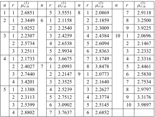
n r µ(r1:n) n r µ( 1)
r:n n r µ( 1)
r:n n r µ( 1)
r:n
1 1 2.6851 5 3.5551 8 1 2.0869 7 2.9118
2 1 2.3449 6 1 2.1158 2 2.1859 8 3.2500
2 3.0252 2 2.2540 3 2.3009 9 3.9225
3 1 2.2307 3 2.4259 4 2.4384 10 1 2.0696
2 2.5734 4 2.6538 5 2.6094 2 2.1467
3 3.2511 5 2.9934 6 2.8363 3 2.2332
4 1 2.1733 6 3.6675 7 3.1749 4 2.3316
2 2.4027 7 1 2.0993 8 3.8478 5 2.4461
3 2.7440 2 2.2147 9 1 2.0773 6 2.5830
4 3.4201 3 2.3525 2 2.1640 7 2.7534
5 1 2.1388 4 2.5239 3 2.2627 8 2.9797
2 2.3113 5 2.7512 4 2.3774 9 3.3176
3 2.5399 6 3.0902 5 2.5145 10 3.9897
4 2.8802 7 3.7637 6 2.6852
Table 1 – Some numerical values generated by the recurrence relations of order statistics from
doubly truncated Makeham distribution.
These special cases are used as initial conditions for generating numerical values for the moments.
We implemented the two recurrence relations (2.1)and(3.1) using Matlab. The first table gives the numerical results for the single moments of order statis-tics for a random sample of sizen = 10 from the doubly truncated Makeham distribution.
Acknowledgement. The authors would like to thank the anonymous referee and the associate editor for their comments and suggestions, which were helpful in improving the manuscript.
REFERENCES
[1] M.I. Hendi, S.E. Abu-Youssef and A.A. Alraddadi, Order Statistics from Doubly Trun-cated Gompertz Distribution and its Characterizations. The Egyptian Statistical Journal,
50(1) (2006), 21–31.
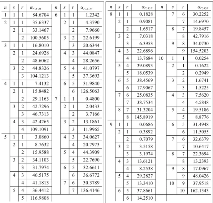
n s r αr;s;n n s r αr;s;n
1 1 1 84.6704 6 1 1 1.2342
2 1 1 35.6337 2 1 4.3790
2 1 33.1467 2 7.9660
2 100.5605 3 2 22.6199
3 1 1 16.8010 3 20.6344
2 1 24.6928 4 3 44.0847
2 48.6062 4 28.2656
3 2 44.8326 5 4 41.0797
3 104.1213 5 37.3693
4 1 1 7.4132 6 5 31.9840
2 1 15.8482 6 126.5063
2 29.1163 7 1 1 0.4800
3 2 42.7296 2 1 2.0433
3 46.7313 2 3.7166
4 3 42.4265 3 2 13.1861
4 109.1091 3 11.9965
5 1 1 3.0860 4 3 34.0627
2 1 8.7632 4 20.7973
2 15.9588 5 4 44.3909
3 2 34.1103 5 22.7690
3 31.7974 6 5 32.6611
4 3 46.5175 6 36.6772
4 41.1813 7 6 30.3789
5 4 36.4412 7 136.4146
5 116.9808
n s r αr;s;n n s r αr;s;n 8 1 1 0.1828 7 6 30.2252 2 1 0.9081 7 14.6970 2 1.6517 8 7 19.8457 3 2 7.0318 8 42.7916 3 6.3953 9 8 34.0730 4 3 22.6896 9 154.5203 4 13.7684 10 1 1 0.0254 5 4 39.0893 2 1 0.1622 5 18.0539 2 0.2949 6 5 38.4569 3 2 1.6741 6 17.9067 3 1.5225 7 6 25.0835 4 3 7.5620 7 38.7534 4 4.5848 8 7 31.3204 5 4 19.5186 8 145.8919 5 8.8776 9 1 1 0.0686 6 5 31.4948 2 1 0.3892 6 11.5055 2 0.7079 7 6 32.6379 3 2 3.5158 7 10.6417 3 3.1974 8 7 22.3694 4 3 13.6121 8 13.2393 4 8.2538 9 8 17.0967 5 4 29.2827 9 48.0426 5 13.3410 10 9 37.9518 6 5 37.8661 10 162.1343
6 14.2510
Table 2 – Some numerical values generated by the recurrence relations of order statistics from doubly truncated Makeham distribution.
[3] N. Balakrishnan and H.J. Malik,Order statistics from the linear-exponential distribution, part I: Increasing hazard rate case.Commun. Statist. Theor. Meth.,15(1) (1986), 179–203.
[4] N. Blakrishnan, H.J. Malik and S.E. Ahmed,Recurrence relations and identities for moments of order statistics, II: Specific continuous distributions. Commun. Statist. Theor. Meth.,
17(8) (1988), 2657–2694.
[5] A.H. Khan and I.A. Khan,Moments of order statistics from Burr distribution and its charac-terizations.Metron,45(1987), 21–29.
[7] A.H. Khan, S. Parvez and M. Yaqub,Recurrence relations between product moments of order statistics. J. Statist. Plan. Inf.,8(1983a), 175–183.
[8] A.H. Khan, M. Yaqub and S. ParvezRecurrence relations between moments of order statistics. Naval Res. Logist. Quart.,30(1983b), 419–441.
[9] M.M. Mohie El-Din, M.A.W. Mahmoud, S.E. Abu-Youssef and K.S. Sultan,Order Statistics from the doubly truncated linear exponential distribution and its characterizations.Commun. Statist.-Simula.,26(1997), 281–290.
[10] M.M. Mohie El-Din, M.A.W. Mahmoud and S.E. Abu-Youssef, Moments of order statis-tics from parabolic and skewed distributions and characterization of Weilbull distribution.