ISSN 0101-8205 www.scielo.br/cam
New approach for tanh and extended-tanh methods
with applications on Hirota-Satsuma equations
HASSAN A. ZEDAN
Mathematics Department, Faculty of Education, Kafr El-Sheikh University Kafr El-Sheikh, Egypt
E-mail: [email protected]
Abstract. In this work, we establish new exact solutions for the Hirota-Satsuma equations. New approach for the tanh is used and extended tanh methods to construct traveling wave solutions in terms of a hyperbolic tangent functions. New families of solitary wave solutions and periodic
solutions are also obtained for Hirota-Satsuma equations. Our approach is reduce the size of
the computational adopted in other techniques without any conditions to apply on any system of partial differential equations.
Mathematical subject classification: 35K99, 35P05, 35P99.
Key words: Tanh method, extended tanh method, Hirota-Satsuma equations, traveling wave solutions, solitary wave solutions.
1 Introduction
The world around us is inherently nonlinear. The Hirota-Satsuma equations are widely used as models to describe complex physical phenomena in various fields of science, especially in fluid mechanics, solid stat physics, plasma physics. Var-ious methods have been used to explore different kinds of solutions of physical models described by nonlinear PDEs. One of the basic physical problems for those models is obtaining their traveling wave solutions. Concepts like solitons, peakons, kinks, breathers, cusps and compacton are now being thoroughly investigated in the scientific literature [1-3]. During the past decades, quite a
few methods for obtaining explicit traveling and solitary wave solutions of the Hirota-Satsuma equations have led to a variety of powerfull methods, such as inverse scattering method [4], bilinear transformation [5], the tanh-sech method [6], Backlund and Darboux transform [7], Hirota [8], tanh-function method [9-10]. Moreover these methods, extended tanh-function method [11-12], modified extended tanh-function method [13-14] and homogeneous balance method [15]. The extended tanh-function method and the modified extended tanh-function method belong to a class of methods called sub-equation method for which these appears few basic relationships among the complicated NLPDEs in the study and some simple and solvable nonlinear ordinary equations.
In this work, we introduce a matrix spectral problem with three potentials and propose a corresponding hierarchy of nonlinear evaluation equations. An interesting equation in the hierarchy is a generalization of the Hirota-Satsuma coupled kdv equations:
ut = 1
2ux x x−3uux +3(vw)x, (1)
vt = −vx x x+3uvx, (2)
wt = −wx x x+3uwx. (3)
2 Tanh method
In this section, we will try to search for a new analytical solutions for system (1)-(3), by using tanh method [12, 16]. This technique has been proven to be very powerful in finding travelling-wave solutions. We represent the tanh method for the problems (1)-(3) which is a workable and universal solution method that can be used to find exact as well as approximate solutions. This technique is based on the fact that in many cases traveling-wave solutions can be written in terms of a hyperbolic tangents.
Let the boundary conditions be
u(x,t)→0, v(x,t)→0; x → −∞ (4)
v(x,t)→v∞, w(x,t)→0; x → ∞ (5)
we get:
c2d 3U(ξ )
dξ3 +6V(ξ ) d W(ξ )
dξ +6W(ξ ) d V(ξ )
dξ
−6U(ξ )dU(ξ ) dξ +2v
dU(ξ ) dξ =0,
(6)
c2d 3V(ξ )
dξ3 −3U(ξ ) d V(ξ )
dξ −v d V(ξ )
dξ =0, (7)
c2d 3W(ξ )
dξ3 −3U(ξ ) d W(ξ )
dξ −v d W(ξ )
dξ =0, (8) where the constants (c and v) represent (positive) wave number and (posi-tive) velocity of the travelling-wave, u(x,t) = U(ξ ), v(x,t) = V(ξ ) and w(x,t)=W(ξ ).
Secondly, substitutingY =tanh ξ into Eqs. (6)-(8) gives:
c2
(1−Y2)2d
3U(Y)
dY3 −6Y(1−Y
2)d2U(Y)
dY2 −2(1−3Y
2)dU(Y)
dY
+6V(Y)d W(Y)
dY +6W(Y) d V(Y)
dY −6U(Y) dU(Y)
dY
+2vdU(Y)
dY =0,
(9)
c2
(1−Y2)2d
3V(Y)
dY3 −6Y(1−Y
2)d2V(Y)
dY2 −2(1−3Y
2)d V(Y)
dY
−3U(Y)d V(Y)
dY −v d V(Y)
dY =0,
(10)
c2
(1−Y2)2d
3W(Y)
dY3 −6Y(1−Y
2)d2W(Y)
dY2 −2(1−3Y
2)d W(Y)
dY
−3U(Y)d W(Y)
dY −v d W(Y)
dY =0.
(11)
whereU(ξ )→U(Y),V(ξ )→V(Y)andW(ξ )→W(Y).
Consequently, the boundary conditions reduce to the conditions with respect to the variable with respect to the variableY:
U(Y)→0, V(Y)→0; Y → −1 (12)
To find an exact solution,we consider a finite expansion ofY in the following form:
U(Y)=
M X
m=0
amYm, V(Y)= N X
n=0
bnYn, W(Y)= H X
h=0
chYh. (14)
Substitution of Eq. (14) into Eqs. (9)-(11) and balancing the highest order deriva-tive terms with the nonlinear terms, gives
M= N =H =2. (15)
Taking account of Eq. (15) with Eq. (14), we obtain
U(Y) = a0+a1Y +a2Y2, (16) V(Y) = b0+b1Y +b2Y2, (17) W(Y) = c0+c1Y +c2Y2. (18) By using Eqs. (12) and (13) into Eqs. (16)-(18), we get:
U(Y → −1) = a0−a1+a2=0
a1 = a0+a2
U(Y) = a0+(a0+a2)Y +a2Y2=(1+Y)(a0+a2Y) U(Y) = A1(1+Y)(1+B1Y); A1=a0, B1= a2
a1
(19)
V(Y → −1) = b0−b1+b2=0
b1 = b0+b2
V(Y) = b0+(b0+b2)Y +b2y2=(1+Y)(b0+b2Y) V(Y) = A2(1+Y)(1+B2Y); A2=b0, B2= b2
b1
(20)
W(Y →1) = c0+c1+c2=0
c1 = −c0−c2
W(Y) = c0−(c0+c2)Y +c2y2=(1−Y)(c0−c2Y) W(Y) = A3(1−Y)(1−B3Y); A3=c0, B3= c2
c1,
(21)
After substitution of Eqs. (19)-(21) into Eqs. (6)-(8), and eliminating terms having equal power inY, we get the following:
3A21+3A21B1−3A2A3B2+3A2A3B3+A1c2+A1B1c2
+A1v−A1B1v=0 (22)
3A21+6A2A3+12A21B1+3A21B12+6A2A3B2B3
+8A1B1c2−2A1B1v=0 (23) 3A21B1+3A21B12+3A2A3B2−3A2A3B3−A1c2−A1B1c2=0 (24) A21B12−2A2A3B2B3−2A1B1c2=0 (25) −3A1A2−3A1A2B2−2A2c2−2A2B2c2−A2v−A2B =0 (26) −3A1A2−3A1A2B1−9A1A2B2−3A1A2B1B2
−16A2B2c2−2A2B2v=0 (27)
−3A1A2B1−6A1A2B2−9A1A2B1B2+6A2c2+6A2B2c2=0 (28)
−6A1A2B1B2+24A2B2c2=0 (29)
3A1A3+3A1A3B3+2A3c2+2A3B3c2+A3v+A3B3v=0 (30) 3A1A3+3A1A3B1−3A1A3B3+3A1A3B1B3
−16A3B3c2−2A3B3v=0 (31)
3A1A3B1−6A1A3B3−3A1A3B1B3−6A3c2−6A3B3c2=0 (32)
−6A1A3B1B3+24A3B3c2=0 (33)
In order to obtainA1, B1, A2, B2, A3, B3, we can solve Eqs. (22)-(33). Conse-quently we get
A1= −2c2, B1= −1, A2= 4c 4
A3, B2=0, B3=0, v =4c 2
. (34)
Substituting the above solution into Eqs. (19)-(21), we have the following ana-lytical solutions:
U(Y) =2c2(1−Y)(1+Y), (35) V(Y) = 4c
4
A3(1+Y), (36)
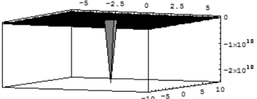
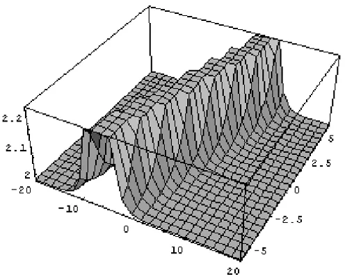
Figure 1 – The graph shows the solution foru(x,t).
To find the wave number(c), we use the boundary condition
V(Y →1) = V∞,
=⇒c2 = 1 4V∞, =⇒v = V∞.
(38)
It is well known that (wave-number)c=109737.3
V∞ = 4.816910004516×10¹⁰, v = 4.816910004516×10¹⁰ Then, Eqs.(1)-(3) have the following analytical solutions:
u(x,t) = −1 2 V∞
1−tanh[c(x−vt)]1+tanh[c(x−vt)], (39)
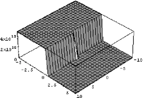
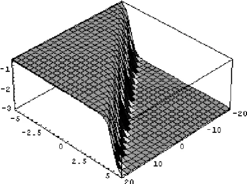
v(x,t) = 1 2V∞
1+tanh[c(x −vt)], (40)
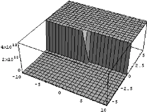
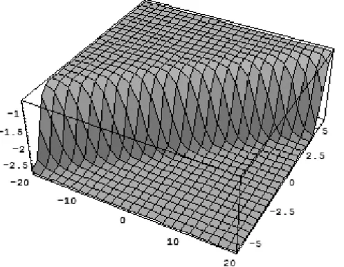
w(x,t) = 1 2V∞
1−tanh[c(x −vt)], (41)
withc, v,V∞, are given.
3 Extended tanh method
Figure 2 – The graph shows the solution forv(x,t).
Using the wave variable ξ = x −ct, Eqs. (1)-(3) reduce to ODEs in the following form:
−cU′ = 1 2U
′′′−3U U′+3(V W)′, (42)
−cV′ = −V′′′+3U V′, (43) −cW′ = −W′′′+3U W′, (44)
where u(x,t)→U(ξ ), v(x,t)→V(ξ ) and w(x,t)→W(ξ ). Integrating Eq. (41) with respect to(ξ ), we get:
−cU = 1 2U
′′−3 2U
2
+3(V W), (45)
where the constant of integration is equal to zero.
The solution of the reduced equations can be expressed as a finite power series inY in the form:
u(x,t) = S1(Y)=
M X
m=0
amY m,
v(x,t) = S2(Y)=
N X
n=0
bnY n, (46)
w(x,t) = S3(Y)=
H X
Figure 3 – The graph shows the solution forw(x,t).
where M, N and H can be determined. By balancing between the highest derivative with the nonlinear terms, in Eqs. (42)-(44) gives
M= N = H =2 (47)
Substituting Eq. (46) into Eqs. (45), we find that:
u(x,t) = S1(y) = a0+a1Y +a2Y2, (48) v(x,t) = S2(y) = b0+b1Y +b2Y2, (49) w(x,t) = S3(y) = c0+c1Y +c2Y2. (50) SubstitutingY =tanh(µξ )in Eqs. (42)-(44), with the aid of Eqs. (47)-(49), and equating the coefficients of each power ofY to zero, we obtain a system of algebraic equations of the parametersa0,a1,a2,b0,b1,b2,c0,c1,c2, namely:
−3a02+2a0c+6b0c0+2a2µ2=0, (51) −6a0a1+2a1c+6b1c0+6b0c1−2a1µ2=0, (52) −3a12−6a0a2+2a2c+6b2c0+6b1c1+6b0c2−8a2µ2=0, (53) −6a1a2+6b2c1+6b1c2+2a1µ2=0, (54)
−3a22+6b2c2+6a2µ2=0, (55)
−3a1b1−6a0b2−2b2c−16b2µ2=0, (57)
−3a2b1−6a1b2+6b1µ2=0, (58)
−6a2b2+24b2µ2=0, (59)
−3a0c1−cc1−2c1µ2=0, (60)
−3a1c1−6a0c2−2cc2−16c2µ2=0, (61)
−3a2c1−6a1c2+6c1µ2=0, (62)
−6a2c2+24c2µ2=0. (63)
Using symbolic software Mathematica to solve the algebraic equations (50)-(62), we obtain the following set of distinct solutions of parameters. The set is given the following cases:
Case 1:
a1 = c1 = b1 = 0
a2 = 4µ2, b2 = 4µ 4 c2
b0 = 1 3
A±B c2
, c0 = 1
12µ4(A±B)c2 c = −3a0−8µ2
where
A = 12a0µ2+24µ4, B = √6µ2
q
(15a2
0+80a0µ2+104µ4) and a0, c2 are arbitrary constants. In this case, the soliton solutions take the form:
u(x,t) = a0+4µ2tanh2µ(x+(3a0+8µ2)t),
v(x,t) = 1 3
A±B c2
+ 4µ 4 c2 tanh
2
µ(x+(3a0+8µ2)t), (64)
w(x,t) = c2
A±B
12µ4 +tanh 2
µ(x+(3a0+8µ2)t)
.
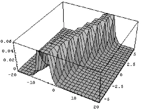
Figs. (4)-(6) represent the soliton solutions for Eq. (63), by taking different values for constants, for examplea0= −1,µ=0.5,c2= −1.
Figure 4 – The soliton solution foru(x,t)in Case 1 whena0= −1,µ=0.5,c2= −1.
Figure 6 – The soliton solution forw(x,t)in Case 1 whena0= −1,µ=0.5,c2= −1.
Case 2:
a1 = b2 = c2 = 0,
a2 = 2µ2, b0 = ±
(a0µ+µ3) c1B
, b1 = 4µ 2(a0
+µ2) c1 ,
c0 = ∓c1A
µB, c = −3a0−2µ 2
,
where
A =
q
−9a02µ2−4a0µ2+4µ4, B = p24a0+24µ2 anda0,c1are arbitrary constants. Thus, the soliton solutions take the form:
u(x,t) = a0+2µ2tanh2µ(x+(3a0+2µ2)t),
v(x,t) = (a0+µ 2) c1
h
±µ B +4µ
2tanh
µ(x+(3a0+2µ2)t)
i
, (65)
w(x,t) = ∓c1A
µB +c1tanh
Figs. (7)-(9) represent the soliton solutions for Eq. (64) as taking different values for constants, for examplea0= −2.5,µ=0.5,c1= −1.
Figure 7 – The soliton solution foru(x,t)in Case 2 whena0= −1.5,µ=0.5,c1= −1.
Figure 9 – The soliton solution forw(x,t)in Case 2 whena0= −1.5,µ=0.5,c1= −1.
Acknowledgement. The author would like to thank the referee for his sugges-tions and comments on this article.
REFERENCES
[1] M. Wadati,Introduction to solitons.Pramana: J. Phys.,57(5-6) (2001), 841–7.
[2] M. Wadati, J. Phys. Soc. Jpn.,32(1972), 1681.
[3] M. Wadati, J. Phys. Soc. Jpn.,34(1973), 1289.
[4] M. Ablowitz and P.A. Clarkson,Soliton, Nonlinear Evolution Equations and Inverse Scatter-ing.Cambridge Univ. Press, New York (1991).
[5] R. Hirota, Direct method of finding exact solutions of nonlinear evolution equations. In: R. Bullough and P. Caudrey (Editors). Backlund transformations. Berlin, Springer (1980). p. 1157–75.
[6] W. Malfliet and W.Hereman, Phys Sprica,54(1996), 569–75.
[7] M. Wadati, H. Sanuki and K. Konno, Prog. Theor. Phys.,53(1975), 419.
[8] R. Hirota, Phys. Rev. Lett.,27(1971), 1192.
[9] E.J. Parkes and B.R. Duffy, Comput. Phys. Commun.,98(1996), 288.
[10] Z.B. Li and Y.P. Liu, Comput. Phys. Commun.,148(2002), 526.
[11] E.G. Fan, Phys. Lett.,A277(2000), 212.
[13] E. Yomba, Chaos, Soliton and Fractals,20(2004), 1135.
[14] E. Yomba, Chaos, Soliton and Fractals,22(2004), 321.
[15] E. Fan and H. Zhang, Phys. Lett.,A246(1998), 403.
[16] A.M. Wazwaz, Chaos, Solitons and Fract.,28(2006), 1005.
[17] A.M. Wazwaz, Comm. in Nonlinear Science and Numerical Simulation,11(2006), 376.
[18] A.M. Wazwaz, Math. and Comput. Modelling,43(2006), 802.
[19] A.M. Wazwaz, Chaos, Solitons and Fract.,28(2006), 454.