Equity Valuation of PANDORA
By
Mafalda Sofia Gomes Luís
Dissertation submitted in partial fulfillment of the requirements for the degree of Master of Science in Business Administration,
at the Universidade Católica Portuguesa
Abstract
This dissertation presents the valuation of PANDORA A/S, traded in the Nasdaq Copenhagen Stock Exchange. For the purpose of the dissertation, first we discuss the different valuation methods, their advantages and disadvantages. As a result, for the valuation itself the DCF method and Relative Valuation were chosen. When applying the DCF valuation method we forecast an enterprise value for PANDORA of DKK130.558 million, an equity value of DKK131.848 million. Thus, the price per share is DKK1.014. Based on this target price PANDORA is undervalued since the current market price is DKK600.50. Additionally, a sensitivity analysis to the riskier components of the valuation was performed to account for the uncertainty tied to the industry and the markets where the company operates. Finally, the price target was compared to the valuation performed by J.P. Morgan Cazenove, published in February 2015, where the recommended price target is DKK650. Even being the conclusion the same, we compare the different assumptions of both models that led to different price targets.
09 March 2015
Supervisor: José Carlos Tudela Martins
i
Acknowledgements
Firstly, I would like to thank my supervisor, Professor José Tudela Martins, for his availability, guidance and advice during the thesis.
Secondly, I must thank those that helped me to search the data used in this work as well as the sharing and continuous discussion of important ideas. In this group I include Tiago Sequeira, Frederico Dias and Francisco Fernandes. Additionally, my friends and co-workers at Jerónimo Martins played a very important role throughout the last months while helping to stay focus for the permanent motivation to deliver the dissertation.
Thirdly, I would like to give a special thanks to André for his important support, helping me to run this marathon by never let me stay behind schedule and for his presence in moments that required more strength to keep the work done.
Last but not least, I would like to thanks to my family and closest friend that somehow made this process more pleasant.
iii
List of Abbreviations
APT Arbitrage Pricing Theory APV Adjusted Present Value ASP Average Sales Price
CAGR Compound Annual Growth Rate CAPEX Capital Expenditure
CAPM Capital Asset Pricing Model COGS Cost of Goods Sold DCF Discounted Cash-Flow DDM Dividend Discount Model DPS Dividend per Share
EBIT Earnings Before Interest and Taxes
EBITDA Earnings Before Interest, Taxes, Depreciation and Amortization
EV Enterprise Value
FCF Free cash flow
FCFE Free Cash Flow to Equity FCFF Free Cash Flow to the Firm GDP Gross Domestic Product LFL Like-for-like
NWC Net Working Capital NIBD Net Interest Bearing Debt
OW Overweight
PVTS Present Value of Tax Shields P/E Price-to-Earnings Ratio
Rf Risk Free Rate
ROIC Return on invested capital
VAT Value-added tax
WACC Weighted Average Cost of Capital
YTD Year to date
v
Index of Graphs
Graphic 1: Expected Global Luxury Sales 2013 – 2018 ... 23
Graphic 2: PANDORA vs SXXP 600 Index stock price evolution (4 October 2010 = 100) ... 27
Graphic 3: Revenue and EBITDA margin ... 27
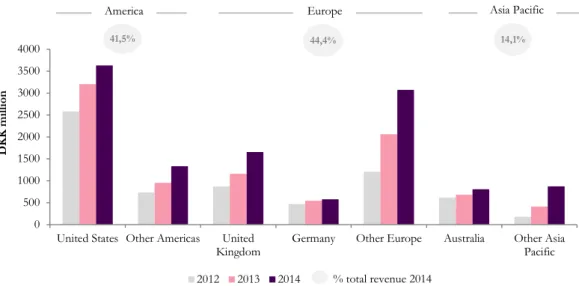
Graphic 4: Revenues breakdown by geography ... 28
Graphic 5: Revenues Breakdown by Product (% total revenue) ... 31
Graphic 6: Operating Costs breakdown (% of revenue) ... 32
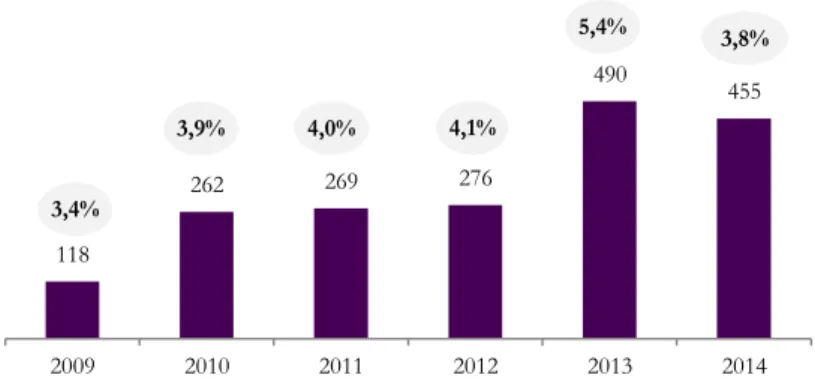
Graphic 7: CAPEX (DKK million and % of revenue) ... 33
Graphic 8: Net Debt Analysis ... 34
Graphic 9: PANDORA’s Revenues by Quarter ... 39
Graphic 10: PANDORA's Revenue Projection (DKK million) ... 40
Graphic 11: PANDORA's Revenue Projection, Breakdown by Geography (% total revenue) ... 41
Graphic 12: PANDORA's Revenue Projection, Breakdown by Product (% of total revenue) ... 43
Graphic 13: PANDORA's Operational Costs Breakdown (DKK million) ... 45
Graphic 14: PANDORA's Capex and Amortizations forecast (DKK million) ... 46
Graphic 15: Operational Working Capital forecast ... 48
Graphic 16: PANDORA’s enterprise value breakdown ... 52
Graphic 17: DCF valuation breakdown ... 53
Index of Tables
Table 1: Number of Points of Sales 2014... 30Table 2: Operational results forecast ... 46
Table 3: PANDORA’s Capex and Amortization forecast ... 47
Table 4: PANDORA’s Operating Working Capital ... 48
Table 5: PANDORA’s expected FCFF ... 50
Table 6: WACC inputs ... 52
Table 7: DCF, sensitivity analysis to critical inputs, share price (DKK) ... 55
vii
Contents
1. Introduction ... 1
2. Literature Review... 3
2.1. Valuation Methods Overview ... 3
2.2. Discounted Cash Flow model ... 4
2.2.1. Cash Flows ... 4
2.2.2. Discount Rate ... 5
2.2.2.1. Cost of equity ... 6
a) Risk Free ... 7
b) Beta ... 7
c) Risk premium ... 9
2.2.2.2. Cost of debt ... 10
2.2.3. Time frame ... 10
2.2.4. Growth rate ... 11
2.2.5. Models description ... 12
2.2.5.1. WACC ... 12
2.2.5.2. APV ... 13
2.2.5.3. DDM ... 14
2.3. Multiples Model ... 15
2.4. Real Options model ... 16
2.5. Multinational companies’ valuation and emerging market’s valuation ... 17
2.6. Conclusion ... 18
3. Industry Review ... 19
3.1. Luxury goods industry ... 19
3.2. Macroeconomic implications ... 20
3.3. Geographic analysis ... 20
3.3.1. Europe ... 21
3.3.2. North America ... 21
3.3.3. Emerging markets ... 21
3.3.4. China ... 21
3.4. Drivers of Growth ... 22
3.4.1. Past growth ... 22
3.4.2. Future growth ... 22
viii
3.4.3. Future of the Industry ... 23
3.5. M&A in the sector ... 24
4. Company Review ... 25
4. 1. PANDORA ... 25
4.1.1. History ... 25
4.1.2. Shareholders ... 26
4.1.3 Overview ... 26
4.1.3.1 Revenues ... 27
A. Revenues by Geography ... 28
B. Revenues by Sales Channels ... 29
C. Revenues by Product ... 31
4.1.3.2 Costs ... 31
A. Capital Expenditures and Depreciations... 33
4.1.3.3 Net Debt ... 33
4.1.3.4 Working Capital ... 34
4.1.4. Risk Parameters ... 35
4.1.5. Future perspectives ... 36
4.1.6 Competitors ... 36
5. Company Valuation ... 39
5.1. Introduction ... 39
5.2. Explicit period length ... 40
5.3. Operational Forecasts ... 40
5.3.1. Revenues ... 40
5.3.1.1 PANDORA’s Revenue by Geography ... 41
5.3.1.2 PANDORA’s Revenue by Product ... 42
5.3.2. Costs ... 43
5.4. Operational results ... 45
5.5. Capex and Amortizations ... 46
5.6. Working Capital ... 47
5.7. Net Debt ... 49
5.8. Valuation ... 49
5.8.1. DCF valuation ... 49
5.8.1.1 Free Cash Flow ... 50
ix
5.8.1.3 DCF Valuation Conclusion ... 52
5.8.1.4 Sensitivity Analysis ... 53
5.8.2. Multiples ... 55
5.8.2.1 Peer Group ... 55
5.8.2.2 Multiples Valuation ... 56
5.8.3. Conclusion ... 57
5.9. Equity Research Comparison ... 57
5.10. Conclusion ... 59
Appendix A ... 61
Appendix A.1 –Balance Sheet as Reported ... 61
Appendix A.2 – Income Statement as Reported ... 62
Appendix A.3 – Revenues Forecast by Geography ... 63
Appendix A.4 – Revenues Forecast by Product ... 64
Appendix A.5 –Balance Sheet Forecast ... 65
Appendix A.6 –Income Statement Forecast ... 66
Appendix A.7 – Detailed Income Statement Forecast ... 67
Appendix A.8 – Detailed Working Capital Forecast ... 68
Appendix A.9 – Detailed Capex Forecast ... 68
Appendix A.10 – DCF valuation ... 69
Appendix A.11–Sensitivity analysis, Growth and Decline scenario ... 70
Appendix B ... 71
Appendix B.1– Research Note ... 71
1
1. Introduction
Over the past few years, the world has experienced a major financial crisis that was followed by a global recession still affecting many economies. In fact, it was considered for most of the experts the worst of the post-war era. During the crisis, the economy struggled and, especially in Europe, the real economy was strongly affected.
In this scenario, a couple of countries in Europe, namely in Northern Europe where countries like Denmark decided to stay out of the Eurozone and let the Krona float freely, had become pockets of resistance where the impact of the recession has been felt less than elsewhere and founded their way to growth. Motivated by searching a growing company in this scenario, PANDORA A/S (“PANDORA” or “company”) appears like an enthusiastic company with a promising future.
The present dissertation is subject to the Equity Valuation theme. Therefore the dissertation’ purpose is to value PANDORA, by carefully presenting the assumptions and adjustments required to establish the fair price target for the company.
The structure of this dissertation is as follow. Firstly, the literature review in Section 2 analyzes the main topics on equity valuation through the discussion of different theories and its usage in the valuation of the chosen company. Section 3, gives some insides over the industry where PANDORA is inserted and Section 4 contains the company overview. Finally, Section 5 contains the valuation of the company along with the corresponding price target and a recommendation, where it is also explained the difference between the value for the company and the one published by a leading investment bank.
3
2. Literature Review
According to Damodaran (2006) “valuation lies at the heart of much of what we do in finance”. Valuation is one of the most discussed topics within the financial world and it plays a key role in transactions and companies’ decisions. However, it can mean different things to different people. Over the years different authors have defined valuation and presented how to compute the value of a specific business using different approaches, ranging from the simplest to the most complicated method but sharing some common characteristics. Thus, in this chapter we will discuss the most well-known methods used in finance including the consistency of the assumptions and their main advantages and disadvantages, then concluding which is the most appropriated on valuing PANDORA.
2.1. Valuation Methods Overview
Over the last years the importance of the valuation of business has been increasing. For the owners and investors it is crucial to answer to the following questions: “How much is the business worth?” and “How it can be more valuable?”. The answer to these questions has changed motivated by different growth drivers and ambitions but the valuation methods have remain very stable.
For the purpose of this dissertation we will use the segregation mentioned by Damodaran (2002) and Young et al. (1999) according to which there are three approaches to valuation. The first, Cash Flow Based Valuation, relates the value of the asset to the present value of the expected future cash flows on that same asset. In this case cash flows are discounted at a risk-adjusted discount rate, usually Weighted Average Cost of Capital (WACC), to arrive at an estimate of value.
The second, relative valuation, estimates the value of the asset by looking at the pricing of the comparable assets relative to a common variable such as earnings, cash flows, book value or sales. This method is commonly known as multiples.
According to some empirical studies the Discounted Cash-Flow (DCF) approach outperform when compared to the multiple valuation method. In this context, the findings of Kaplan and Ruback (1995 and 1996) suggest that both the DCF and the multiple approaches add relevant information to the company valuation. However, DCF method appears to produce lightly better results. Nevertheless, given today’s economic environment, forecasting revenues and cash flows for a long period seems to be more difficult. As a result, the combination of both methods gives an extra inside about the true value of a company. Finally, the third method, contingent claim valuation, uses option pricing models to measure the value of assets that share option characteristics.
4
This method is often called real options and was initially used to value traded options but there has been more recently an attempt to extend the reach of these models into more traditional valuation.
Young et al. (1999) states that no single approach is expected to be consistently more reliable than others. Thus, it is important to take into consideration the available data, the nature of the company and the assumptions of each model to ensure that we use the most appropriated method.
2.2. Discounted Cash Flow model
The basic cash-flow based models are WACC, Adjusted Present Value (APV) and Dividend Discount Model (DDM model), all of them presented later in detail.
The DCF valuation is based upon expected future cash flows and discount rates. As so, this approach is to be used for companies whose cash flows are currently positive and can be estimated with some reliability for future periods and expected to remain positive. The mentioned assumptions are an important limitation of the models.
The DCF model outputs the enterprise value and the equation is as follow:
( ) ∑
( )
( ) ( )
Additionally to the cash flows forecast the important features to compute the enterprise value are: terminal growth rate (g), explicit period (n) and which discount rate to use, all being developed in the following chapters.
The method is based on the work produced by Modigliani and Miller (1958) where the authors argue that the firm’s value should be the division of the expected profit before deduction of interest by the rate of return of the company. As a matter of fact, after this approach many academics developed a cost of capital that takes into account the different capital employed in the firm.
2.2.1. Cash Flows
The value of an asset comes from its capacity to generate cash flows. The first step is to estimate the earnings generated by a firm, the second is to estimate the portion of this income that would go towards taxes and finally, the third is to develop a measure of how a firm is reinvesting back for future growth (working capital and capital expenditure). This approach demonstrates the sum of the cash flows to all claimholders in the firm.
5
The Free Cash Flow to Equity (FCFE) reflects the equity value of a company and how much cash being generated by company’s operations a firm can afford to return to its stockholders.
( )
FCFE Model is also known as a model that discount potential dividends instead of actual dividends (DDM Model detailed later).
The Free Cash Flow to the Firm (FCFF) is basically the FCFE not deducted from the net debt payments or taxes, Copeland et al. (2000), so being based upon after-tax operating earnings.
( ) ( )
The differences between FCFF and FCFE arise primarily from cash flows associated with debt. Net debt payments might be important for some models where interest tax shield is a distinctive part of value, for instance, when the future tax savings is risky because the company may become non-taxpaying.
Put simply, as referred by Damodaran (2006) one way to approach DCF valuation is to value the equity stake in the business, usually called equity valuation, considering the cash flows after debt payments and reinvestments, FCFE and discount at cost of equity. The alternative to equity valuation is to value the entire business that is obtained by discounting the FCFF at the weighted average cost of capital. The last is known as Firm DCF model and takes into consideration the tax benefits of debt and expected additional risk associated with debt.
2.2.2. Discount Rate
To measure the value of operations, we should discount each year’s forecast of free cash flow for time and risk. Koller et al. (2010) state that in any company free cash flow must be available to all investors and consequently, the discount factor must represent the risk faced by all investors.
Independently of the DCF model chosen, the essential is that they all need a discount rate. A key insight from finance theory is that the use of capital imposes an opportunity cost on investors since funds are diverted from earning a return on the next best equal-risk investment. As referred by Bruner et al. (1998) since investors have access to a host of financial market opportunities, corporate uses of capital must be benchmarked against these capital market alternatives. The cost of capital provides this benchmark.
The discount rate takes into account the time value of money and the risk or uncertainty of the future cash flows.
6
Accordingly, it should always compensate the investor for the opportunity cost of investing in a particular asset instead of another with the same risk and time condition Copeland et al (2000). The discount rate should be applied accurately to the specific case of each company and to the cash flows to be computed. Thus, depending on the origin of the cash flows, from equity or debt, they should be discounted respectively to the cost of equity or the cost of debt.
2.2.2.1. Cost of equity
Several methods are available to calculate the cost of capital for a specific investment. Three of the more common models are Capital Asset Pricing Model (CAPM), Fama-French Three Factor Model and Arbitrage Pricing Theory (APT).
Using the portfolio theory, Sharpe (1964) placed risk into two categories, systematic risk and unsystematic risk. Systematic risk referred to as Beta ( ), is the risk of being in the market, and cannot be diversified. Unsystematic risk is the risk that is specific to each individual company CAPM comes from capital markets and assumes that prudent investors will eliminate unsystematic risk by holding large and well-diversified portfolios. The CAPM model assumes that there are no transaction costs, all assets are traded, investments are infinitely divisible and there is no private information. Thus, the cost of capital that is the rate of return that investors require to invest in the equity of a company can be defined as follow:
(4) ( )
To use the CAPM model we need three inputs, namely, that is the risk free rate, is the risk premium and represents the systematic risk a specific asset has when compared to the market, which has a systematic risk of 1. Then, according to Sharpe (1964) the expected rate of return demonstrates a constant relationship between expected return and systematic risk. Although, Fama and French (xxx) demonstrate that the CAPM model is too simple and that other variables should be added to the model to find the correct rate of return, namely size, book to market and momentum. On the other hand, the APT model is built on the simple idea that two investments with the same exposure to risk should be priced to earn the same expected return.
Additionally, as mentioned by Bruner et al. (1998) the cost of capital should be the current costs reflecting current financial market conditions, not historical or sunk costs to allow to equal the investors’ anticipated internal rate of return on future cash flows.
However, based on the results of Kaplan and Ruback (1995 and 1996) that run evidence that DCF valuation methods provide reliable estimates of market value, CAPM will be the method explained in this literature review and used later on for PANDORA’s valuation.
7
a) Risk Free
According to Damodaran (2008b, 2010b) some asset might be considered as risk free if they met several conditions, namely no default risk, which generally implies that the security has to be issued by a government and no uncertainty about reinvestment rates which implies that there are no intermediate cash flows (zero coupon bond). In this context, a risk free investment that requires neither default nor reinvestment risk is long term government bond rates: default-free zero coupon.
Ideally, the risk free asset should be adjusted for each cash flow in different periods. However, this is not completely feasible. Then, to choose the government bond to use it is important to match up the maturity with the cash flows occurrence as much as possible. According to Koller et al. (2010) an investor should look for long-term government bonds in the use of a risk free rate.
Typically, US or German bonds can be considered as default-free government bonds for US valuations and European valuations, respectively. However, as Koller et al (2010) highlight it is crucial to use government bonds yields denominated in the same currency as the firm’s cash flows.
Nowadays, after the sovereign-debt crisis it becomes harder to find what can be called a risk free asset. Nevertheless, the most famous Rating Agencies (Fitch, Standard & Poors and Moody’s) publish regularly the ratings of each country sovereign debt that can be used to define which ones are the riskless assets.
In Europe, the standard and the most suitable approach would be German government bond adding up the default risk premium related with the rating of the country at the time of the valuation. Thus, in PANDORA’s valuation the German Bonds cannot be used since PANDORA’s Cash flows are in Danish Krone (DKK). Thus, according to Damodaran (2010b), one should consider the Danish bonds added up with default risk premium.
b) Beta
The CAPM relates the expected return on a stock to its beta, the systematic risk or non-diversifiable. So, the accuracy of the cost of equity estimates relies on the accuracy of the beta estimate. It seems reasonable to consider that a company use both debt and equity to finance its assets which has profound implications in the likelihood of the equity investors in case of bankruptcy. Hence, it is necessary to consider two CAPM’ equations depending on the mix structure of the firm, levered or unlevered.
8
Later in this literature review we will confirm that the levered formula should be used in the WACC method, where we assume that the company has a mix capital structure, and that the unlevered equation should be used in the APV method where the firm is only equity financed.
( ) ( ) ( ) ( )
If we assume that the debt carries no market risk, thus having a beta of zero, according to Damodaran (2002) the beta of equity alone can be defined as a function of the unlevered beta and the debt-equity ratio:
( ) ( ( )
As we have seen, beta is a standardized measure of the risk that an investor adds to the market portfolio and statistically this added risk is computed by the covariance of the market with the asset. The computation of a beta is defined by Ross (1976) as the covariance of an investment and the market performance, normalized by the variance of the market return. After, Koller et al. (2005) defines the computation of the beta as a simple regression between the company stock returns and a diversified portfolio.
Furthermore, the beta represents the only firm-specific input in the CAPM model and the only one requiring estimation. As so, one can conclude that the only reason for a firm to have a different expected return from another is because both have different betas.
Damodaran (2002) refers three different approaches for the computation of beta.
First, the historical market beta that is a common approach for publicly traded companies, where one estimate returns that an investor would have made investing in an equity interval, such as a week or month, and then related to the returns on an equity market index. However, as mentioned by the author the length period estimation, the definition of the return period and the chosen market index used to compare can be difficult.
On the other hand, one can also use a service beta. The beta provided by Bloomberg is one of them and have the particularity of given details about the computation of the adjusted beta, which is estimated as follows:
( )
Bloomberg uses price appreciation in the chosen stock and the market index in estimating betas. However, they ignore dividends which can have a huge impact in companies that pay no dividend or when the dividends are significantly higher than the market.
On the other hand, the usage of the adjusted beta of Bloomberg is very important particularly in cases where comparison with comparable peers is not possible.
9
Nevertheless, one of the issues of the historical betas is that is depending on the firm’s financial leverage in the past that can diverge from future options.
The second approach is the fundamental betas that rely less on historical betas and is more on intuitive underpinnings of betas. In this case, the author presents another way to compute the beta, called Bottom-up Beta, where there is no need to use past prices.
This approach includes the flowing process as defined: 1) identifying the business that make up the firm, 2) estimate the average unlevered betas for publicly traded firms, peer group of the company, 3) calculate the unlevered beta for the firm and take a weighted average of the unlevered betas using the proportion of firm value derived from each business as the weights, 4) calculate the current debt to equity ratio for the firm using market values if available and, finally, 5) estimate the levered beta for the equity in the firm using the unlevered beta and the debt to equity ratio computed before.
Finally, the third approach is to estimate the beta of a firm or its equity from accounting earnings instead of the traded price. However, this approach is not recommended due to the possible manipulation of the accounting earnings, the impact of non-operating factors in the accounting earnings and the time frame of measurement, usually quarterly.
c) Risk premium
Equity risk premium is one of the master pieces of CAPM theory and the perspective to this subject has changed over time. Finance theory says that equity market risk premium should equal the excess return expected by investors on the market portfolio relative to riskless assets. However, measures expected future returns on the market portfolio is one of the problems left to solve. According to Sharpe (1964) the risk premium in the CAPM measures the extra return that would be demanded by investors for shifting their money from a riskless investment to the market portfolio or risky investment, on average.
In CAPM model, one of the assumptions is that the market is a perfect benchmark having a beta of 1, thus making the price of risk simply the difference between the market return and the risk free rate.
Damodaran (2011) consider three approaches to estimate the equity risk premium, namely, survey investors and managers to get a sense of their expectations about equity returns in the future, historical approach and implied premiums.
The first approach is, according to Damodaran, the one that has weaker prediction power. The historical premium approach, which remains the standard approach to estimating equity risk premiums, is simple.
10
However, this method has some important limitations and the author points out three reasons: different time periods for estimation, differences in risk free and market indices and differences in the way in which returns are averaged over time.
Even if an investor agree that historical risk premium are the best estimates of future equity risk premiums, one can still disagree about how far back in time to go.
The second issue is based on the risk free chosen, because the risk premium is larger when estimated relative to short term government securities than when estimated against long term bonds. In relation to this topic, Damodaran conclude that the risk free rate chosen in computing the premium has to be consistent with the risk free rate used to compute the excess return. Finally, analyzing the consensus in corporate finance and valuation theory the argument for using geometric average premiums as estimates seems stronger.
The problem with any historical premium approach is that is backward looking. Thus, Damodaran propose a new approach, implied equity premiums by equity prices, assuming that the market, overall, is correctly priced, reflecting a forward-looking approach.
Bruner et al. (1998) conducted a survey concluding that most of the best-practice companies’ use a premium of 6% or lower and Koller et al. (2010) argue that the market risk premium should be in between 4.5% to 5.5% range.
2.2.2.2. Cost of debt
According to Hitchner (2006) the cost of debt is the actual rate a company pays on interest-bearing debt, the pretax cost of debt, assuming that the company is borrowing at market rates. It is the theoretical cost that the company should bear to issue new debt. However, when there is long-term debt, the rates being paid now may differ from the prevailing market due to changes in required yields on debt of comparable risk.
Since the interest paid on debt instruments is tax deductible, the cost to the company does not include this part. The after-tax cost to the company represents its effective rate.
( )
2.2.3. Time frame
An important part of DCF valuation is how to estimate when the firm will reach “stable growth”. When doing a DCF valuation, at a certain point predicting year-by-year, called the explicit period, becomes impractical. As so, when the key drivers of the valuation are considered to be stable it is possible to use perpetuity based continuing value, Koller et al (2010). The same authors recommend a use of an explicit period of 10 to 15 years. However it’s difficult to forecast for such a long period. Nevertheless, explicit period should be just enough to allow the company to reach a steady state.
11
Additionally, Myers (1974) proved that increasing the number of years of projections can decrease the error incurred in the assumptions, especially in the case of an incorrect discount rate. Hitchner (2006) defines terminal value as the value of the business after the explicit or forecast period. The terminal value, generally referred as residual value, is of considerable importance as it often represents a substantial portion of the total value of any company. The perpetual growth rate used in terminal value should be aligned with the GDP long-term growth rates or inflation where the company being evaluated is inserted.
On this subject, Kaplan and Ruback (1995) mentioned that the terminal value can be obtained using a terminal capital cash flow and assuming a constant nominal growth rate in perpetuity. The authors argue that the company will be, in this case, in what one can call stable growth. Thus, the cash flow should be normalized when the company is in a situation of constant and equal investment, meaning that the CAPEX equalize the Depreciations and Amortizations.
2.2.4. Growth rate
The most popular view nowadays is that a company must grow to survive and prosper. However, growth creates value only when a company generates returns on invested capital Koller et al. (2010). How to achieve the balance between the two aspects is critical.
The average industry revenue growth changes considerably across industries and drivers are different. Koller et al. (2010) consider three main components in the overall growth rate: Portfolio momentum, market share performance and mergers and acquisitions. Portfolio momentum is the organic revenue growth a company enjoys because of the overall expansion in the market segments represented in its portfolio whereas market share performance is the organic revenue growth a company records by gaining or losing share in any particular market. Sustainable growth is difficult to accomplish because most product markets have natural life cycles. Growth can accelerates as more people want to buy the product, until it reaches its point of maximum penetration Koller et al. (2010). However, as highlighted by Damodaran (2006) the growth rate used in the model has to be less than or equal to the growth rate in the economy. In the specific case of PANDORA, a company that is still expanding to new markets and launching new products it seems reasonable to consider that the company remains as a growing company far from its maximum penetration in the market.
According to Hitchner (2006) there is often a need to identify companies capable of “sustainable growth” that is, a level of continued growth that a firm can reasonably be expected to sustain over the long term. As a long-term sustainable growth one can use between 3 and 6 percent, depending on the underlying characteristics of the company and its future prospects.
12
On the other hand many analysts use the anticipated inflation rate, which has average approximately 3 percent historically assuming no real growth in the underlying business
The expected growth rate in earnings and cash flows is a key input when valuing a company, Damodaran (2008a). The same author present several alternative to try to estimate the expected earnings growth.
The first is by looking at the historical growth, which raises some problems since it is by definition a backward looking approach. Second, for publicly traded firms one of the most common sources of expected earnings growth rates is to look to the equity research analysts who follow the firm, which could be biased and present some substantial error. Finally, the author looks into the fundamentals of growth, reinvestment and the return on capital on these investments or improved efficiency. So the expected growth rate is defined as the reinvestment rate multiplied by the return on capital.
Thus, for the purpose of PANDORA’s valuation and assuming that the company will reaches steady state after a certain number of years and starts growing at a stable growth rate after that,
gn, the value of the firm can be computed as in formula (1).
2.2.5. Models description
2.2.5.1. WACC
The WACC blends the rates of returns required for both of debt holders and equity holders since the different sources of financing required a different return. WACC is an average figure used to indicate the cost of financing a company’s asset base. Thus, WACC should be used in companies that are financed with debt and equity and is defined as follow:
( )
( ) Where:
Re - cost of equity, Rd - cost of debt
E – Market Value of the firm’s equity D – Market Value of the firm’s debt T – Tax rate
Academics and investors have a strong preference for WACC-based models, considering that the discount rate WACC works best when a company maintains a relatively stable debt-to-value ratio.
13
There are different assumptions about the debt level. Modigliani and Miller (1963) assume that the level of debt is constant. Therefore, the value of the WACC is constant over time. On the other hand, Miles and Ezzel (1980) and Harris and Pringles (1985) assume that the level of debt is rebalanced continuously so as to maintain a constant debt ratio. Moreover, as the level of debt is always proportional to the value of the unlevered firm, the expected return on the tax shield is the same as the cost of capital of the unlevered firm which implies a constant WACC.
2.2.5.2. APV
Modigliani and Miller (1958) develop the model assuming that a company’s choice of financing structure will not affect the value of its economics assets. Only market imperfections, such as taxes and distress costs affect the company’s value. However, the ideal world defined by the authors is not completely true. Then, as taxes exist the valuation of a company may need to account for changes in ratio of debt relative to value, because it keeps changing over time. The DCF model usually discounts the future cash flows at a constant WACC. However, if the company planned to change its capital structure significantly, namely by paying down the debt as cash improves, is lowering their future debt-to-value ratios. In these cases we should turn to an alternative model, APV that separates two different components: the value of tax shields from debt financing and the value of operations as if the company were all equity financed.
Cooper and Nyborg (2007) explain the APV model by first assess the firm’s unlevered value, meaning discounting the firm’s operating FCF at the unlevered discount rate and then making a separate calculation of the present value of the debt tax shields. The way to compute the present value of tax shields (PVTS) is to multiply the corporate tax rate by the market value of debt. In simple terms, the APV approach considers the value of the company without debt and then adding debt to the firm we should consider the up and down side of debt, thus including tax benefits since interest expenses are tax deductible and the increase in bankruptcy costs, as follows:
( )
If a company’s debt-to-value is expected to change it is recommended to use the APV model that specifically forecasts and values any cash flows associated with the capital structure separately, rather than embedding their value in the cost of capital Koller et al. (2010)
When using this model, the assumption is that the company is completely equity financed and the discount rate should be the unlevered cost of equity. Nevertheless, is important to state that when applied correctly, APV or WACC method reach identical values, in the majority of the cases.
14
2.2.5.3. DDM
The simplest model for valuing equity is the DDM model and its primary attraction is its simplicity and its intuitive logic. As point out by Damodaran (2006) the only cash an investor receive from a firm when buy publicly traded stock is the dividend. Then, the value of a stock is the present value of expected dividends on it.
The model consists in two types of cash flows, the dividends during the period an investor holds the stock and an expected price at the end of the holding period. However, since the expected price is itself determine by future dividends, the value of a stock is the present value of dividends through infinity. Thus, the DDM model follows the following equation that reflects the expected dividend per share (DPS) and the cost of equity:
( ) ∑ ( ) ( )
There are two main inputs in this model, cost of equity and expected dividends. The cost of equity is usually computed through the CAPM. To obtain the expected dividends per share one must make assumptions about expected future growth rates in earnings and payout ratios. In this sense, Gordon developed the Gordon Growth Model that can be used to value a firm that is in “steady state” with dividends growing at a rate that can be sustained forever, and is the simplest one but is too dependent on the inputs for the growth rate.
However, this model can only be used in firms where an investor is expect for a limited number of stable and high-dividend paying stock. On the other hand, the DDM model is based upon the premise that the only cash flows received by stockholders are dividend. However, stockholders can afford also the cash flows left over after meeting all financial obligations, including debt payments and after covering capital expenditure and working capital needs. In this case the DCF model is more accurate.
Comparing the DDM model with FCFE model one can obtain the same value under two conditions. The first, when dividends are equal to the FCFE and the second when the FCFE is greater than dividends but the excess cash (FCFE minus dividends) is invested in projects with Net Present Value of zero.
As mentioned, DDM Model is a simple model to value directly the equity stake in a company but it presents severe limitations. The most relevant one is related with dividends manipulation. Being based in dividends the valuation can be biased since companies can chose to hold back cash and do not distribute dividends to build large piles of cash in their balance sheet.
15
On the other hand companies can also chose to distribute always the same amount of dividends to shareholders in order to not disappoint shareholders even if they are not generated through cash flows from the company but instead from raise of debt. In this case, the valuation through DDM model would be too optimistic. As a result, this model will not be used to value PANDORA.
2.3. Multiples Model
One alternative to discounted cash flow models is relative valuation or multiples. Damodaran (2008a) defined relative valuation as an approach to find assets that are cheap or expensive relative to how similar assets are being priced by the market in the moment. Moreover, Koller et al. (2010) argue that multiples are a very useful tool to understand the expectations of the market about the industry and the companies. Following the same line of thoughts, Fernandéz (2001) argues that multiples valuation should be used after applying another valuation model to analyze the information and the main differences between the company being valued and its comparable firms. Many other authors agreed with this idea, and so multiples as valuation method will only be used as a completary method for PANDORA’s valuation.
According to Damodaran (2006) a comparable firm is one with cash flows, growth potential and risk similar to the firm being valued. This approach becomes more difficult to apply when the sector of activity is very fragmented or composed by few firms. By using a group of comparable companies one can place the DCF model in the proper context. If the market is, on average, correct the DCF valuation and relative valuation should converge in the conclusion.
However, applying multiples valuation method can be a challenge. Not only we need to choose the most suitable peer group for the company but also which multiple to use.
According to Goehart et al. (2005) the first step is to identify the company’s industry players and then apply the four basic principles to have proper multiples: use peers with similar prospects for ROIC and growth, use forward-looking multiples, use enterprise-value multiples as they are less susceptible to manipulation by changes in capital structure.
Also, Liu et al. (2001) provided some additional evidence on forward-looking multiples concluding that they are more accurate than historical multiples which might seem coherent because expected future cash flows reflect better the future prospect of the company than historical cash flows.
One of the important justifications for paying higher values, or multiples, of earnings or book value for some firms than others is the growth rate expected for future cash flows, Damodaran (2008).
16
Generally, there are two types of commonly used types of multiples analysis, comparable transactions and multiples for publically listed companies. In the first, the valuation occurs looking to transactions that have taken place in the market for comparable companies. However, multiples for publically listed companies seems more appropriated for PANDORA since it is a public listed company and it is possible to find some comparable listed companies. Thus, there are different multiples and the most commonly used are the Enterprise Value (EV) to EBITDA and Price-to-Earnings ratio (PER).
EV-to-EBITDA is considered for several authors to be a good multiple when compared to others, since it is less susceptible to changes in the capital structure of the firm and to non-operational cash-flows like amortizations and depreciations and extraordinary debt payments. On the other hand, PER despite being one of the most used multiples have received some critiques. First, PER considers earnings, an accounting figure that might be different from country to country when applying different accounting rules and they change over time. Second, it includes non-cash items and does not take into consideration the capital structure of the companies. Moreover, it only applies for companies with positive Earnings Per Share (EPS) Thus, for the purpose of PANDORA’s valuation we will use both mentioned multiples.
Saying that, after the peer group formation and all the assumptions met apply multiples is a simple task. It is just the multiplication of the operational indicator that we chose to use for the peer group multiple. To illustrate the EV-to-EBITDA and PER formulas are presented below:
( )
( )
2.4. Real Options model
Scholes and Merton developed a model that avoids the need to estimate either future cash flows or the cost of capital. The model relies on a replicated portfolio for securities. Given the success of this approach more recently there have been attempts to translate the concepts of replicating portfolios to corporate valuation. As long as one can find a suitable replicating portfolio, there is no need to discount future cash flows. However, replicating portfolios for companies and their projects are difficult to create and today’s applications are limited. Frequently this model is used in Oil & Gas industry or mining companies. As so, for the purpose of this dissertation this model will not be used.
17
2.5. Multinational companies’ valuation and emerging market’s valuation
Valuing companies that spread their business into different countries or segments present additional challenges to valuation. Furthermore, if a company is present in emerging markets, something that comes immediately to mind is the expected existence of an additional risk. Some of the risks associated with those countries are related with war, corruption, expropriation and the volatility associated can damage the operating results of the company. However, within the academics and finance world there is no consensus on how to adjust these risks.
Damodaran (2004) admits the use of a country risk premium that should be added to the market risk premium in order to adjust the discount factor since the country risk premium cannot be, according to the author, diversifiable. To estimate the risk premium one could use sovereign ratings provided by Rating Agencies. On the other hand, Koller et al. (2010) recommend the adjustment of cash flows rather than adjusting the discount rate as proposed by Damodaran since they believe that the country risk premium can be diversifiable.
Additionally, if a company has different business segments what one could expect is an impact on the beta of the company. Another particular question is related with the tax rate to use or the currency or exchange rate to valuing the company.
As Damodaran (2009) mentioned, the different risk, growth and cash flow profiles of the cash flow streams generated by multinational companies requires us to reconsider how to estimate discount rates and approach valuation.
One of the approaches is to consider the company as a whole, using the weighted average of the risk parameters and consider the consolidated cash flows. However, this approach can easily fail since the inputs in the discount rate and cash flows can have themselves differences within the countries. As so, the author presented us “The light side of valuation” where the computation and assumptions for the inputs in the DCF model are modified in order to include all the characteristics of multinational firms. If the information is available one should use the disaggregated figures to value the business separately.
The second alternative that Damodaran presents is to use the relative valuation, trying to find comparable firms, but within the segments or countries in which the company operates. As so, the author has developed some best practices in what concerns with the main inputs to the model to this specific type of valuations.
Taking this into consideration for PANDORA’s valuation, due to the lack of information available related to different geographies where the company operates namely in terms of costs and investments, the valuation will be performed considering the company as a whole and the discount rate will be computed as if the company don’t operate in emerging market.
18
However, higher discount rate and different revenues will be taken into consideration out in the sensitivity analysis to have a better look to the impact in the company.
2.6. Conclusion
After seeing the most relevant literature review it is possible to conclude which are the best models to apply in the case of PANDORA’s valuation, in accordance to their characteristics. In terms of Cash Flow based models, DCF method is the method chosen to use to value PANDORA since the company has a very stable capital structure. Moreover, when applying the DCF method we will take into account reasonable scenarios in addition to the base valuation case to understand the impact of critical variables on the price target of the company.
The explicit forecast period considered will be just the enough to account for all the expected operational changes in the company and take into consideration the strategic objectives and investment plans.
The APV method will not be used since it applies best when companies are expecting some changes in their capital structure, which is not the case of PANDORA. Also the DDM model presented before was not chosen to apply in case of PANDORA because it is easily manipulated by companies’ decisions. A company might decide to pay constant dividends over the year not supported by operational results or by holding back cash to build large pills of cash in the balance sheet without distributing dividends. Moreover, PANDORA’s dividend policy is expected to change, since PANDORA announced higher dividends in the following years. Additionally, we will use the relative valuation based on forward looking multiples, the ones considered to be more acceptable. The multiples chosen are Enterprise Value to EBITDA ratio and Price Earnings ratio. First, is an easy method to use and allows us to have a good understanding of the industry and PANDORA’s main competitors. Second, this method could help us to validate the conclusions of other methods. Nevertheless, we need to bear in mind that this valuation method assumes market efficiency and it relies on the chosen peer group, which can have a huge impact on the final conclusion.
19
3. Industry Review
3.1. Luxury goods industry
The luxury goods industry embrace companies with a value chain that starts in development, production, distribution, market and finally selling apparel, jewellery, watches, leather goods and accessories.
The definition of luxury is not easy to agree on. In fact, in the recent past this definition has become even harder since companies are expanding many luxury items into the hands of masses through lower prices. However, the industry itself is frequently defined according to the luxury pyramid that consists of three different segments.
First, the absolute luxury segment is characterized mainly by storied heritage, exclusive distribution, highest quality product and the highest price in their respective category. The positioning is to generate a sense of exclusivity and uniqueness where the brand’s emotional environment attached is extremely important and advertising is not used. As a matter of fact, Europe has a higher concentration of absolute luxury brands. Some well-known examples placed in this segment will be Hermes and Brioni. In terms of price segment it would be higher than $3.000 price tag.
Second, aspirational luxury segment, sits in the middle of the pyramid and is more concentrated in distinctiveness and more convenient prices. In this case, advertise plays a support role in the communication of the brand that is driven by public relations and events. The middle segment has been the most affected by the macroeconomic slowdown of the last years. Examples of this segment are Gucci and Yves Saint Laurent. The price range change from $500 to $3.000.
Finally, the accessible luxury segment includes companies like Coach and Tiffani & Co., with prices below $500, is focused on affordability, status and membership component. The communication with clients’ needs to be constant and the focus is on the performance characteristics of the product which can be accomplished by advertising.
Taking into consideration the charactheristics of the industry, PANDORA is within the accessible luxury segment.
Furthermore, the luxury goods industry includes mostly companies that are family-controlled or even family-owned. Thus, profits, brand and human resources are managed with a long-term vision and not necessarily the next-quarter. This different approach is sometimes difficult to investors to overcome when companies chose to sacrifice the next-quarter result in favor of the long term strategy. In cases of listed companies, like Burberry and Tiffany, with a free float of 100%, the growth has been made through acquisitions.
20
Some of the most well-known characteristics of the industry are high operational margins, solid generation of cash and a considerable exposure to the emerging markets. In what concerns to the modus operandi of the majority of the companies in this industry, it is common to be retail-driven meaning that companies sell their own jewellery in their own stores.
3.2. Macroeconomic implications
The luxury goods industry was believed to be crisis proof and a highly profitable sector. However, the recession of 2008 was more than a crunch on demand, it was a dramatic change. The dynamism of the luxury goods industry over the past five years, after the hard period of crisis, was driven by the existence and development of brands positioned at accessible prices, which combines with new middle-class in the emerging markets. On the other hand, the world market is ripening and also the luxury industry is evolving accordingly.
Being an industry dependent in the fluctuation of the raw materials used the performance can be highly affected, namely in what concerns EBITDA margins. Some companies have chosen to reflect the price fluctuation to clients through changes in selling prices. Over the last months some of the most used raw materials in jewellery industry, gold and silver, impacted positively the margins.
In what concerns stock performance of the listed companies in the industry, the historical growth is strong. Nevertheless, the doubt is in the sustainability of the stock performance.
3.3. Geographic analysis
Luxury goods companies’ headquarters are mainly located in Europe and USA. Until this point, luxury has been connected with mystique, rich, and heritage that are yet characteristics associated with the old continent. However, new opportunities to grow are in the emerging markets. Therefore, US and European companies have shifted to take advantage of opportunities in emerging countries and have been especially keen to raise their profile in Asia-Pacific countries.
The crisis hit with less intensity the emerging markets since they were affected only indirectly. Nevertheless, for companies into luxury industry it can be a challenge to expand into small but high-growth markets while they need to protect also the foundations in the epicenters of luxury. The differentiation between countries and regions presented later in this chapter will focus, for some of them, on significant differences among the global luxury market and its consumer distribution by nationality, based on a report published by Bain & Company in January 2014, called “Lens on the worldwide luxury consumer”. In this report the consumer base is, in 2013, 330 million people and the luxury market for the same period is of €217 billion in value.
21
For the company to be assessed the regions that really matter in what concerns the company’ activity and future investments are, Europe, North America and Emerging Markets with a specific focus on China.
3.3.1. Europe
According to Euromonitor International, Europe includes five of the top ten luxury markets in the world, that are Italy, France, UK, Germany and Spain.
According to Bain & Company report mentioned before, Western Europe has approximately 80 million consumers and Eastern European countries another 20 million consumers.
In 2013 the spending per capita in the Western Europe, the second biggest market in the world, was of approximately €450, and represented 24% of the total consumers and only 17% of the luxury market since the spending per capital is lower than the average.
3.3.2. North America
North America remain as the largest luxury market in the world with a consumer base of approximately 90 million people, which represents 27% of the luxury consumers in the world but only 17% of the total market in terms of value, with one of the lowest spending per capita of approximately €400. It is interesting to notice that the USA represents alone more than one quarter of global sales.
3.3.3. Emerging markets
Some of the emerging markets to be considered in luxury market are China, Russia, Brazil and India. Some of these countries or other developing countries have faced a deceleration of growth in the last couple of years after a period of extreme growth. In emerging countries like India and Brazil the growth rate have been held up by regulatory issues, like restrictions to withdraw the profits.
These countries have improved in their governance, competitiveness and demographics and the outlook persist very positive for the future. In the following years, emerging markets are expected to have strong economic growth and to contribute positively to the luxury goods industry in terms of consumption and production.
3.3.4. China
In 2010, China was the world’s fifth largest luxury market which demonstrates an incredible growth process over the last years. According to Bain & Company, the Chinese’ market has approximately 50 million people, being within the top three in 2013 in terms of consumer base. China has grown to become the world’s largest jewellery market with a market value of DKK 487 billion in 2013, according to the Annual Report of 2013 of Pandora.
22
China is now the third largest consumer based, with 14% of the total consumers in luxury market, and the second highest spending with 28% of the total market value, meaning that is one of the biggest countries in terms of spending per capita, approximately €1.250, only preceded by Middle Eastern with a spending per capita of €1.400.
Additionally, Bain & Company states that, in 2013, 67% of all Chinese luxury purchases were made overseas. Moreover, according to Euromonitor International, 2013, The State of the Luxury
Market, “luxury spending in China is rising steeply”. But establishing operations in China is not
an easy task and companies have faced a stumbling block.
3.4. Drivers of Growth
Given the constant evolution of the luxury industry there are some interesting changes that had led the companies to growth in the past and are now taking place as a driver of growth and are capable of shape the industry in the future.
3.4.1. Past growth
The luxury goods industry was driven by the exposure to emerging markets, not only by the presence in those countries but also through tourism and purchases in developed countries. According to a report recently published by Mckinsey in 2014, titled “The jewelry industry in 2020”, most of the growth came from the expansion of established jewelry brands.
3.4.2. Future growth
As for future trends, companies start to integrate the whole business, through value chain integration, from design to sourcing of raw materials, to production, marketing and distribution. The objective is to control the quality and the service level to customers to be able to protect the brand. It is expected that the majority of the luxury good companies will enjoy restrict control over all aspects of their business.
Secondly, the online sales have increased and the omnichannel is starting to get some influence. Even companies that were originally averse to the internet, and have struggled to sell online given their concern about exclusivity and prestige, are now using their websites to communicate fashion shows, stories and important factors for the business and customer.
According to Euromonitor International, in 2013, e-commerce sales of luxury goods represented 5.3% of total luxury goods sales, which reflects an increase of 23% since 2008. As a direct result of increasing control over the business, the direct retail and also e-commerce operations are becoming one of the most important figures of the distribution model. Over the last several years, a revolution in the luxury industry has occurred due to the rise of the social media and mobile applications.
23
Third, the market is now much more demanding in terms of collections and speed of delivery. What started by Inditex’s phenomena is now one of the most important trends that companies need to deal with. Consumers are pressing for innovation. On the other hand, products are now copied much faster, which means that companies need to build some kind of temporary monopolies, toward innovation, to compete in the market at the first place. Additionally, the rise of men’s luxury is another tendency that could influence the market in the near future.
And finally, up to this time, brand image was one of the most important variables for the luxury business but consumer behavior changed and now quality sometimes means more than brand image. After the crisis consumers became less concern in acquiring status since they became more aware of the value of money.
3.4.3. Future of the Industry
The prospect for the industry seems to be very tempting. For instance, according to The State of
the Luxury Market, 2013, from Euromonitor International, the global luxury sales until 2018, is
expected to behave as follow.
Graphic 1: Expected Global Luxury Sales 2013 – 2018
Source: Euromonitor International
According to the same source, developed markets will continue to be the largest spenders and in 2018 the emerging markets are expected to account for almost 30% of sales.
To put it simply, luxury industry is one of most attractive industries in the market nowadays. According to a study performed by Bain & Company called “Luxury Goods Worldwide Market
Study Winter 2014”, published in January 2014, “the number of luxury consumers worldwide was
more than triples over the past 20 years, from roughly 90 million consumers in 1995 to 330 million at the end of 2013”. The same report mentioned that the number of consumers in the market is expected to rise up to 400 million luxury consumers worldwide by 2020 and 500 million by 2030. This boost represents 10 million new consumers per year.
230 240 250 260 270 280 290 300 310
2013E 2014E 2015E 2016E 2017E 2018E
us $ B ill io n
24
Moreover, based on interviews to twenty executives at global jewellery companies, analysis of public data and annual reports of the same companies, Mckinsey (2014), in the report The
Jewellery Industry estimates that in 2020 the sales of the jewellery industry will totalize
approximately €250 billion, which represents a growth rate of 5 to 6 per cent each year, driven by the new appetite for jewellery. According to Euromonitor International report in 2013 the luxury jewellery is roughly €60 billion.
To face the demand of affordable luxury goods, a significant number of high profile luxury goods companies have shift down market, reorganize their portfolio to have products to support their core business at more accessible prices.
This shift in segments that are common across all industry, though having also companies going upmarket, will lead to a completed segmented market. In the future it is reasonable to expect that affordable luxury will work as a standalone industry.
On the other hand, the expertise and distribution channels will continue to be crucial characteristics in the industry.
3.5. M&A in the sector
Having survived a recession and experienced a change in consumer demand in 2011, a number of luxury firms were in a position to make opportunistic acquisitions.
The enthusiasm for European and American brands in emerging markets is strong and growing, motivating many luxury goods companies to expand their international expansion, particularly in Asia and the Middle East. At the same time, buyers and investment groups in emerging markets are looking for western brands. Thus, one of the most active buyers of luxury brands are private equity firms that play a crucial role in providing the necessary capital to help young brands to grow.
Additionally, as mentioned before, as companies are going through vertical integration process the M&A activity has been increasing and takes place at both ends of the value chain.
On the other hand, for the big conglomerates M&A activities has also increase toward the consolidation of the business, by expanding to other complementary businesses to gain scale and own expertise.
25
4. Company Review
4. 1. PANDORA
4.1.1. History
PANDORA was founded in 1982 as a wholesaler, importing from Thailand, aiming to offer women across the world high quality, modern and genuine jewellery at low prices. A couple of years after, as a result of the increasing demand, the focus changed to direct clients in Denmark. In 1987, the wholesale business was discontinued. In 1989 the company decided to start in-house production in Thailand. Over the following years PANDORA start to expand to other markets and today is a distinctive brand that just in 30 years went from a local jeweler in Denmark to a world-leading international company.
In 2000 PANDORA launch the charm bracelet concept that is now the most well-known product. The first concept store opened in 2006 and now the company has more than 800 concept stores, most of them operated by franchisees. As mentioned by PANDORA, the company does not distinguish between own and operated stores and stores driven by franchisees.
PANDORA is present in more than 90 countries, over 9.900 points of sale, through a retail category concept ranging from Concept stores, Shop-in-Shop and Gold stores to Silver and White multi-brand stores.
Since 5 October 2010 PANDORA shares have been listed on the Nasdaq Copenhagen Stock Exchange. At the end of 2014 PANDORA operate more than 1.400 concept stores, 251 of them owned by the company, and 70 owned shop-in-shops. PANDORA employs over 11.400 people worldwide, of whom than 7.900 are based in Thailand, where the company manufactures its jewelry.
The company has established a well-defined brand within the luxury segment and one of the most recognized characteristics of the company in the market respects to its appealing store design and store environment that is uniform across all markets. Currently, PANDORA has 6.2 million members of PANDORA club, an online VIP area for the most enthusiastic customers that according to the company helps to build a strong sense of brand loyalty. PANDORA controls every step of the value chain of almost all jewellery products from in-house design to production and also distribution of jewellery products to sales channels through own distribution subsidiaries, third party distributors and directly operated stores. The vertically integrated business model includes i) Design & Development ii) Forecast & Production iii) Communication & Launch iv) Sell & Replenish and v) Distribution & Service.