Assessing static and dynamic response variability due to parametric uncertainty on fibre-reinforced composites

(1)

Article

Assessing Static and Dynamic Response Variability

due to Parametric Uncertainty on Fibre-Reinforced

Composites

Alda Carvalho1, Tiago A.N. Silva2ID _{and Maria A.R. Loja}3,_*ID

1 _{Grupo de Investigação em Modelação e Optimização de Sistemas Multifuncionais (GI-MOSM),}

Instituto Superior de Engenharia de Lisboa, CEMAPRE, ISEG, Universidade de Lisboa, 1200-781 Lisboa, Portugal; acarvalho@adm.isel.pt

2 _{Grupo de Investigação em Modelação e Optimização de Sistemas Multifuncionais (GI-MOSM),}

NOVA UNIDEMI, Faculdade de Ciência e Tecnologia, Universidade Nova de Lisboa, 2829-516 Caparica, Portugal; tan.silva@fct.unl.pt

3 _{Grupo de Investigação em Modelação e Optimização de Sistemas Multifuncionais (GI-MOSM),} IDMEC-Instituto Superior Técnico, Universidade de Lisboa, 1049-001 Lisboa, Portugal

* Correspondence: amelialoja@dem.isel.ipl.pt; Tel.: +351-962-564-688

Received: 31 December 2017; Accepted: 26 January 2018; Published: 1 February 2018

Abstract: Composite structures are known for their ability to be tailored according to specific operating requisites. Therefore, when modelling these types of structures or components, it is important to account for their response variability, which is mainly due to significant parametric uncertainty compared to traditional materials. The possibility of manufacturing a material according to certain needs provides greater flexibility in design but it also introduces additional sources of uncertainty. Regardless of the origin of the material and/or geometrical variabilities, they will influence the structural responses. Therefore, it is important to anticipate and quantify these uncertainties as much as possible. With the present work, we intend to assess the influence of uncertain material and geometrical parameters on the responses of composite structures. Behind this characterization, linear static and free vibration analyses are performed considering that several material properties, the thickness of each layer and the fibre orientation angles are deemed to be uncertain. In this study, multivariable linear regression models are used to model the maximum transverse deflection and fundamental frequency for a given set of plates, aiming at characterizing the contribution of each modelling parameter to the explanation of the response variability. A set of simulations and numerical results are presented and discussed.

Keywords:response variability of composites; parametric uncertainty characterization; multivariable linear regression models; composite laminates; static and free vibration analysis

1. Introduction

In a global perspective, the growth verified in the usage of composite materials may be attributed mainly to the transportation and construction industries, although in other areas such as medical and health technologies they are becoming more relevant. Within the manufacturing processes, some are witnessing a higher development; namely, resin transfer moulding (RTM) and glass-mat-reinforced thermoplastics (GMT), as well as the long-fibre-reinforced thermoplastics (LFRT) [1]. According to the composites industry report for 2017 [2], since 1960 the composites industry has grown 25 times, whereas the aluminium and steel industries grew less than 5 times. These numbers denote an important reality landscape on the increasing use of composite materials, confirming a continuous need for deeper holistic research to enhance the understanding of these kinds of materials [3].

(2)

The need for materials with better mechanical properties has already led to the development of glass fibres—most often used as reinforcement—with a tensile strength 2–3 times higher than the traditional ones for fulfilling specific operation requirements, such as those posed by the blades of wind turbines, bicycle frames, and the diverse automotive and aerospace parts. Simultaneously, lightweight materials have become very attractive as they simultaneously meet regulatory requirements for emission reduction, fuel economy and safety. For instance, in the automotive and aerospace industries, carbon-fibre-reinforced polymers (CFRP) have been the primary beneficiary. However, the cost of carbon fibres still constitutes a disadvantage and these materials are not fully recyclable at the end of their life cycle.

The use of composite materials in the most diverse areas poses different questions depending on the nature of the specific application. Moreover, the great heterogeneity intrinsic in the constitution of these kinds of materials in conjunction with the usual manufacturing processes is deemed to be responsible for the significant variability in the structural responses when compared to those of a structure made of homogeneous traditional materials, such as metals, for instance.

Attempting to consider this uncertainty and to assess its effects using different approaches, several published works can be found. Mesogitis et al. [4] presented a review about the multiple sources of uncertainty associated with material properties and boundary conditions. In this work, the authors presented numerical and experimental results concerning the statistical characterization and influence of uncertain inputs on the main steps of the manufacturing process of composites, including defects induced by the process itself.

In the context of more focused work, we refer to Noor et al. [5] who proposed a two-phase approach and a computational procedure for predicting variability in the nonlinear responses of composite structures associated with variations in the geometric and material parameters of the structure. To this aim, the authors considered a hierarchical sensitivity analysis to identify the parameters with greater influence on the responses. After this screening stage, the selected parameters were fuzzified and a fuzzy set analysis was performed to determine the variability of the responses.

The problem of uncertainty propagation in composite laminate structures was studied by António and Hoffbauer [6]. They considered an approach based on the optimal design of composite structures to achieve a target reliability level. In this work, the uniform design method (UDM) was used to study the space variability using a set of design points generated over a design domain centred on the mean values of the random variables. An artificial neural network (ANN) was developed based on supervised evolutionary learning with the input/output patterns of each UDM design point. This ANN was used to implement a Monte Carlo simulation (MCS) procedure to obtain the variability of the structural responses. The use of ANN was also considered by Teimouri et al. [7] to investigate the impact of manufacturing uncertainty on the robustness of commonly used ANN in the field of structural health monitoring (SHM) of composite structures, namely concerning the thickness variation in laminate plies. The ANN SHM system was assessed through an aerofoil case study based on the sensitivity of location and size predictions for delamination with noisy data. Mukherjee et al. [8] studied the influence of material uncertainties in failure strength and reliability analysis for single- and cross-ply laminated composites subjected to only axial loading. These authors have categorized the uncertainty at different scales, although in [8] they only considered ply level uncertainties. Note that these uncertainties are included as random variables and the strength parameters of the composite are derived through uncertainty propagation considering both Tsai-Wu and maximum stress criteria. MCS was performed to quantify the effect of those uncertain parameters. In [9], the authors were concerned with the prediction of the uncertainty induced by the manufacturing process on the effective elastic properties of long fibre-reinforced composites with a thermoplastic matrix. Carvalho et al. [10] studied the uncertainty propagation in functionally graded material (FGM) plates with an approach that can be viewed as the precursor of the present work.

In the present work, the goal was to study the uncertainty propagation of laminate material properties as well as geometric parameters related to the thickness and fibre orientation or stacking

(3)

angle of each ply. These modelling parameters have specific contributions to the simulated linear static response and, therefore, on the characterization of its variability. To enable the simulation of uncertainty on the modelling or input parameters, a random multivariate normal distribution was used to generate the set of input parameters, ensuring independence. The obtained results intend to enable a more comprehensive understanding of the influence of uncertain modelling parameters on the variability of structural responses.

2. Materials and Methods 2.1. Fibre-Reinforced Composites

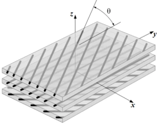
The typical configuration of laminated fibre-reinforced composite material is illustrated in Figure1 where an exploded view of generic three-layered laminate with arbitrary ply orientation angles is presented.

J. Compos. Sci. 2018, 2, x FOR PEER REVIEW 3 of 17

static response and, therefore, on the characterization of its variability. To enable the simulation of uncertainty on the modelling or input parameters, a random multivariate normal distribution was used to generate the set of input parameters, ensuring independence. The obtained results intend to enable a more comprehensive understanding of the influence of uncertain modelling parameters on the variability of structural responses.

2. Materials and Methods

2.1. Fibre-Reinforced Composites

The typical configuration of laminated fibre-reinforced composite material is illustrated in Figure 1 where an exploded view of generic three-layered laminate with arbitrary ply orientation angles is presented.

Figure 1. Exploded view of a three-layered fibre-reinforced composite material.

In Figure 1, the laminate in-plane directions are denoted by x- and y-directions; also visible is the angle θ defined between the positive senses of the fibre longitudinal direction within each ply and the y-direction. The possibility of considering different materials for different plies, allied to the ability to vary the stacking angles of each ply, allows to some extent for customized materials that result in structures with improved mechanical performance.

In the present work, the study focused on a carbon fibre-reinforced composite material that is available in the market, the properties of which are given in Table 1.

2.2. Constitutive Relations and Equilibrium Equations

Due to the characteristics of the plate structures to be analysed, the first-order shear deformation theory of plates and shells (FSDT) will be considered. Accordingly, the stress–strain relationships for each ply in the laminate coordinate system can be written as:

σ σ σ = Q Q Q Q Q Q Q Q Q ε ε γ ; σ σ = Q_Q Q_Q γγ (1)

with the transformed reduced elastic stiffness coefficients given in the literature [11,12]. The coefficients σ stand for the stress tensor components and ε and γ represent the normal and total shear strains, respectively. To overcome the through-thickness constant prediction of the transverse shear stresses, a shear correction factor of 5/6 is considered.

To obtain the equilibrium equations required for linear static and free vibration analysis, the Lagrangian functional is considered:

L = U + V − T (2)

where U denotes the elastic strain energy, V the potential energy of the external transverse applied loads and T the kinetic energy. Considering Hamilton’s principle [11,13,14] we have:

Figure 1.Exploded view of a three-layered fibre-reinforced composite material.

In Figure1, the laminate in-plane directions are denoted by x- and y-directions; also visible is the angle θ defined between the positive senses of the fibre longitudinal direction within each ply and the y-direction. The possibility of considering different materials for different plies, allied to the ability to vary the stacking angles of each ply, allows to some extent for customized materials that result in structures with improved mechanical performance.

In the present work, the study focused on a carbon fibre-reinforced composite material that is available in the market, the properties of which are given in Table1.

Table 1.Carbon fibre prepreg laminate properties (IM7/8552 UD Hexcel composites).

E11(GPa) E22, E33(GPa) G12, G13(GPa) G23(GPa) ν12, ν13 ν23 ρ(kg/m3)

161 11.38 5.17 3.98 0.32 0.44 1500

2.2. Constitutive Relations and Equilibrium Equations

Due to the characteristics of the plate structures to be analysed, the first-order shear deformation theory of plates and shells (FSDT) will be considered. Accordingly, the stress–strain relationships for each ply in the laminate coordinate system can be written as:

   σ_xx σyy σxy   =    Q11 Q12 Q16 Q12 Q22 Q26 Q16 Q26 Q66       ε_xx ε_yy γ_xy   ; " σyz σxz # = " Q44 Q45 Q45 Q55 #" γ_yz γ_xz # (1)

(4)

with the transformed reduced elastic stiffness coefficients given in the literature [11,12]. The coefficients σ_ijstand for the stress tensor components and εiiand γijrepresent the normal and total shear strains,

respectively. To overcome the through-thickness constant prediction of the transverse shear stresses, a shear correction factor of 5/6 is considered.

To obtain the equilibrium equations required for linear static and free vibration analysis, the Lagrangian functional is considered:

L=U+V−T (2)

where U denotes the elastic strain energy, V the potential energy of the external transverse applied loads and T the kinetic energy. Considering Hamilton’s principle [11,13,14] we have:

δ

t2

w

t1

(U+V−T)dt=0 (3)

After the functional minimization and some mathematical manipulations, the free vibration and linear static equilibrium equations for a discretized domain can be written as:

(K−ω2_iM)q_i=0

Kq=F (4)

where M is the mass matrix, K represents the elastic stiffness matrix of the structure, F denotes the generalized load vector and q represents the generalized degrees of freedom vector. The i-th natural frequency is represented by ωiand qiis the corresponding mode shape. Regarding a set of boundary

conditions, it is possible to obtain the nodal generalized displacements.

2.3. Simulation of Modelling Parameters Uncertainty

The variable responses from a set of real specimens were simulated by considering the uncertainty in the material and geometrical properties of a laminated composite. In the present work, we focused on the study of the uncertainty propagation on the material properties, ply thicknesses and stacking angles. Each modelling parameter has a specific effect on the simulated response, either static or dynamic, and therefore on the characterization of their variability. Thus, to simulate the uncertainty in the material and geometrical properties, a set of modelling parameters X was sampled from a multivariate normal distribution. Hence, the modelling parameters were sampled considering X ∼N(µ,Σ); that is, X is distributed as a normal variable with the mean values µ (Table1) and the covariance matrixΣ. Additionally, the correlation matrix, equal to the identity, is given to ensure independence among the modelling parameters. Note that a Latin hypercube sampling (LHS) with the ability to ensure the independence between variables [15] was used to sample 30 observations from a multivariate normal distribution. This sample size is not a rule but a guideline. It is a good compromise in the sense that it was sufficient to support the significance of the results while keeping the problem at a reasonable size for dealing with experimental test data.

2.4. Forward Propagation of the Uncertainty

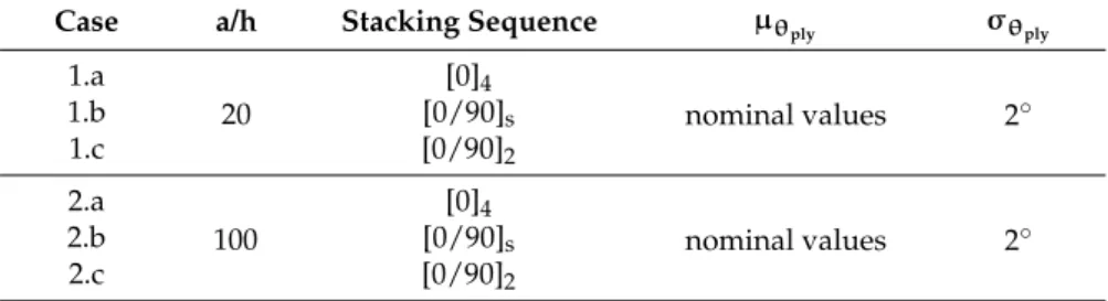
The sampling procedure was carried out to obtain different samples, aiming at simulating several plates made of different combinations of properties that are used with different aspect ratios(a/h); note that a stands for the length of the plate edge and h for its thickness. The mean values of the material properties of the composite materials used are given in Table1. Tables2and3summarize the case studies concerning the stacking angles and individual thicknesses. After obtaining the samples for all the defined case studies, we computed the necessary finite element analysis to evaluate the maximum transverse deflection and a set of natural frequencies, followed by an assessment of the correlation coefficients obtained for all case studies. It is important to note that the uncertain parameters were simulated with a coefficient of variation (CoV) of 7.5% for all the material properties

(5)

(see nominal values in Table 1) and ply thicknesses (Table 3). Regarding the stacking angles, we considered a standard deviation of 2 degrees (Table2).

Table 2.Case studies with uncertain stacking angles(θ_ply).

Case a/h Stacking Sequence µ_θ_ply σθply 1.a 20 [0]4 nominal values 2◦ 1.b [0/90]s 1.c [0/90]2 2.a 100 [0]4 nominal values 2◦ 2.b [0/90]s 2.c [0/90]2

Table 3.Case studies with uncertain ply thicknesses(hply).

Case a/h Stacking Sequence µ_h_ply CoVhply 3.a 20 [0]4 0.131 mm 7.5% 3.b [0/90]s 3.c [0/90]2 4.a 100 [0]4 0.131 mm 7.5% 4.b [0/90]s 4.c [0/90]2

It is important to mention that the sample for the modelling parameters was the same for all the case studies related to the stacking angles. For the cases related to the uncertain ply thicknesses, another sample was used but again it was the same for all the related cases. This was done to enhance the comparison between case studies.

2.5. Multivariable Linear Regression Model

As mentioned, the response variability of the laminated composite plates may be due to the uncertainty associated with several materials and geometrical parameters. Thus, the use of a multivariable linear regression model allows for the use of a probabilistic substitute model with less computational cost. Therefore, for a specific structural response Y, the maximum deflection or a natural frequency and regarding a set of predictors X, which can be material and geometrical properties, the model is generally given as:

Y=β₀+β₁X1+. . .+βkXk+ε (5)

where subscript k is the number of independent variables used to explain the dependent variable Y. The coefficients βirepresent the regression coefficients and ε is the residual or error term. The coefficient

β₀is the intercept that corresponds to the value predicted for the structural response Y when the independent variables are zero. The remaining regression coefficients represent the partial slopes, which denote the influence of an independent variable Xion the response Y. The residual ε is assumed

to follow a normal distribution with a zero mean and constant variance σ2denoted as ε ∼N(0, σ). It is also relevant to mention that the independent variables Ximust be uncorrelated. Therefore, if these

model assumptions are validated, a response prediction ˆy can be estimated from the sampled values xi

with a random residual. The residual ε=y−ˆy can thus be used to estimate the regression coefficients and to validate the model assumptions using the method of least squares [16].

Such a probabilistic model is a multivariable linear regression model. Based on a specific sample, it is possible to determine estimates for each regression coefficient βi, as well as for the coefficient

(6)

by the regression model. The R2coefficient and the adjusted R2(Adj. R2) are outputs of the linear regression model.

According to inferential statistics, the sampled results can be generalized to the population. The analysis of variance (ANOVA) provides the significance of the model based on the p-value of the F-test. If the model is significant, it means that at least one of the slopes is nonzero; thus, we can conclude that the predictors considered in the model are relevant. Under these conditions, the t-test gives the significance of each individual independent variable or model parameter. Moreover, it is possible to construct confidence intervals for the slopes. Once the model has been chosen, the assumptions must be verified for the residuals to assess the validity of the model [16].

3. Results and Discussion

The results presented in the present Section are focused on the assessment of the influence of the parameter uncertainty on the maximum transverse displacement wmaxand on the fundamental

frequency f1of a carbon fibre-reinforced composite plate. Based on the methodology presented in

Section2.3, the material and geometrical properties were simulated using a sample of 30 observations, as referred. With the sampled modelling parameters, we carried out a set of finite element analysis to build a sample of the maximum transverse displacement and natural frequencies for each of the cases identified in Section2.4. The finite element analysis was carried out using nine-node quadrilateral plate finite elements based on the FSDT as described in Section2.2. In the linear static analysis, a unitary uniform transverse pressure loading was applied. In all the presented case studies, the plate is simply supported. Note that the reference to a ply number is related to the stacking sequence order illustrated in Figure1, where the first ply is the lower one considering an ascending stacking order. Unless stated otherwise, the aspect ratio (a/h) of the plates was set to 20.

The results for the different case studies are discussed based on the analysis of the correlation coefficients obtained for different plates and uncertain parameter sets. In the following matrix plots, significance codes were used to ease the results interpretation. Thus, absolute values of correlation coefficients above 0.30 are marked with “*”, above 0.50 with “**” and above 0.75 with “***”.

3.1. Uncertainty in the Material Properties

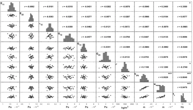
The first case was focused on characterizing the influence that uncertain material properties may have in the maximum transverse displacement and natural frequencies of the plate. To this purpose, we assumed that the plates were built from a unique unidirectional composite layer with the material properties’ mean values presented in Table1. In this case study, the stacking angle was assumed to be unaffected by uncertainty, whereas the material properties and the total thickness of the plate, considered as a single layer, were deemed to be uncertain. Hence, if the referred modelling parameters vary, it is possible to compute the scatter plots of both parameters and responses and the respective correlation coefficients, as well as their histograms. These results are organized in the matrix plot of Figure2.

As a first observation, it is important to conclude on the independence among the modelling parameters, which present a Gaussian pattern with nearly null linear correlation coefficients among each other and consistent scatterplots. This was expected according to the uncertainty simulation described in Section2.3.

From the matrix plot of Figure2, it is possible to conclude that the responses are highly correlated (0.85), which was an expected result. It is also important to note the influence of the plate thickness, which plays a very significant role here for both responses: the maximum deflection (0.95) and the fundamental frequency (0.80). Although with a lower significance, the fundamental frequency is correlated with the density (−0.37) and with the longitudinal elasticity modulus(E11)(0.36). Besides

the plate thickness, only the elasticity modulus is slightly correlated with the maximum deflection with a correlation coefficient of 0.25.

(7)

Considering now the static analysis of the unidirectional composite plate where all modelling parameters are uncertain, a set of correlation coefficients between each of the material and geometrical parameters and the maximum transverse displacement, along with the corresponding scatter plots, are presented in Figure3. Note that in Figure3the different cases for different sets of uncertain parameters are considered; all means that all of the modelling parameters are uncertain, as in Figure2; all hply (fix) means that all modelling parameters are uncertain except the ply thickness, which is kept at its nominal value; the cases where a single property is identified means that only that parameter is uncertain and all the others are kept at their nominal values.J. Compos. Sci. 2018, 2, x FOR PEER REVIEW 7 of 17

Figure 2. Matrix plot of the modelling parameters and the resulting maximum deflection (w ) and

fundamental frequency (f ) (unidirectional plate, a/h = 20, all input parameters uncertain).

Considering the first row of the matrix plot in Figure 3 where all of the modelling parameters are uncertain, we conclude that all the parameters except the density (1.00) are responsible for explaining, to some extent, the whole variability in the transverse displacement. This was an expected conclusion as in a static analysis situation the self-weight of the plate is discarded; the density parameter does not influence the maximum deflection of the plate.

It is important to note the high influence of the plate thickness, which presents a high correlation value (0.96) to the maximum deflection. As seen in Figure 2, the longitudinal elasticity modulus (E ) is the second most significant parameter, although with a correlation coefficient much lower than the one corresponding to the ply thickness. As the ply thickness has the highest influence on the mechanical response of the plate, we proceeded to another study where this modelling parameter was fixed to its nominal value and only the remaining ones could vary. This study aimed to improve the understanding of the relative importance of the other parameters. The results are presented in Figure 4.

If the ply thickness is not affected by uncertainty, it is possible to observe in Figure 4 that in these conditions the longitudinal elasticity modulus (E ) presents a very high correlation (0.99) with a maximum deflection of the plate. It is also a significant parameter concerning the fundamental frequency, although in this case the correlation coefficient between the fundamental frequency and the material density is higher, −0.79 against 0.61. An inverse correlation (minus sign) is observed between the density and the fundamental frequency, as expected.

Another interesting result concerns the correlation between responses. Although they present a significant correlation, this value is not as high as when the thickness was deemed to be uncertain.

Figure 2.Matrix plot of the modelling parameters and the resulting maximum deflection(wmax)and fundamental frequency(f1)(unidirectional plate, a/h = 20, all input parameters uncertain).

Considering the first row of the matrix plot in Figure3where all of the modelling parameters are uncertain, we conclude that all the parameters except the density (1.00) are responsible for explaining, to some extent, the whole variability in the transverse displacement. This was an expected conclusion as in a static analysis situation the self-weight of the plate is discarded; the density parameter does not influence the maximum deflection of the plate.

It is important to note the high influence of the plate thickness, which presents a high correlation value (0.96) to the maximum deflection. As seen in Figure2, the longitudinal elasticity modulus(E11)

is the second most significant parameter, although with a correlation coefficient much lower than the one corresponding to the ply thickness. As the ply thickness has the highest influence on the mechanical response of the plate, we proceeded to another study where this modelling parameter was fixed to its nominal value and only the remaining ones could vary. This study aimed to improve the understanding of the relative importance of the other parameters. The results are presented in Figure4.

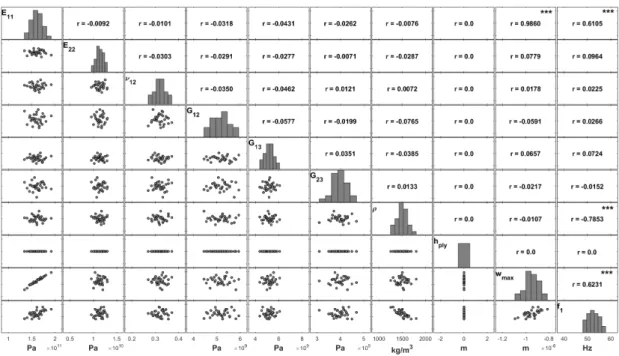
If the ply thickness is not affected by uncertainty, it is possible to observe in Figure4that in these conditions the longitudinal elasticity modulus(E11)presents a very high correlation (0.99) with

a maximum deflection of the plate. It is also a significant parameter concerning the fundamental frequency, although in this case the correlation coefficient between the fundamental frequency and the material density is higher,−0.79 against 0.61. An inverse correlation (minus sign) is observed between the density and the fundamental frequency, as expected.

(8)

Another interesting result concerns the correlation between responses. Although they present a significant correlation, this value is not as high as when the thickness was deemed to be uncertain.

Figure 3. Matrix plot of the maximum deflection (w (m)) for different sets of uncertain parameters (unidirectional plate, a/h = 20).

fundamental frequency (f ) (unidirectional plate, a/h = 20, all modelling parameters uncertain except the ply thickness).

3.2. Uncertainty in the Layer Orientation

In this section, we considered that the plate was built from a laminate with four layers, as already mentioned in Section 2.4. In the first stage of analysis, we assumed that the stacking angles of each layer are affected by uncertainty. The computed results are presented in Figure 5, which presents the sampled values for a set of laminated plates modelled according to Case 1.a (Table 2).

Figure 3.Matrix plot of the maximum deflection(wmax(m))for different sets of uncertain parameters (unidirectional plate, a/h = 20).

Figure 3. Matrix plot of the maximum deflection (w (m)) for different sets of uncertain parameters (unidirectional plate, a/h = 20).

fundamental frequency (f ) (unidirectional plate, a/h = 20, all modelling parameters uncertain except the ply thickness).

3.2. Uncertainty in the Layer Orientation

In this section, we considered that the plate was built from a laminate with four layers, as already mentioned in Section 2.4. In the first stage of analysis, we assumed that the stacking angles of each layer are affected by uncertainty. The computed results are presented in Figure 5, which presents the sampled values for a set of laminated plates modelled according to Case 1.a (Table 2).

Figure 4.Matrix plot of the modelling parameters and the resulting maximum deflection(wmax)and fundamental frequency(f1)(unidirectional plate, a/h = 20, all modelling parameters uncertain except the ply thickness).

3.2. Uncertainty in the Layer Orientation

In this section, we considered that the plate was built from a laminate with four layers, as already mentioned in Section2.4. In the first stage of analysis, we assumed that the stacking angles of each

(9)

layer are affected by uncertainty. The computed results are presented in Figure5, which presents the sampled values for a set of laminated plates modelled according to Case 1.a (TableJ. Compos. Sci. 2018, 2, x FOR PEER REVIEW 2). 9 of 17

Figure 5. Matrix plot of the stacking angles (θ1–θ4) and the resulting maximum deflection (w ) and fundamental frequency (f ) for Case 1.a (a/h = 20, [0]4).

As already mentioned in the previous case study, the individual histograms show a Gaussian behaviour for the stacking angles, which are uncorrelated between themselves as shown by the scatterplots and the corresponding correlation coefficients. It is again relevant that the correlation coefficients related to the modelling parameters are close to zero (Figure 5), which means that their independence is verified. This is consistent with the uncertainty simulation described in Section 2.3.

From Figure 5, we conclude that the stacking angles with higher correlations to the maximum transverse deflection are the first three in the stacking, although there is not a significant predominance from a statistical point of view. It is also visible that the angles of the inner layers provide an inverse effect when compared to those of the outer layers.

To assess in a more detailed way the influence of each ply, we computed several combinations and considered different sets of uncertain parameters. These sets assumed that all the stacking angles are uncertain (All) and that only one ply at a time would have an uncertain orientation (θ1–θ4), as shown in Figure 6. Note that the sample with the maximum transverse displacement given in Figure 5 is the one in Figure 6 with the combination of all stacking angles being uncertain (All).

Figures 6 and 7 present the same study for moderately thin and thin unidirectional plates, respectively. The presented matrix plots show different varying patterns for the maximum transverse displacement. Both figures show that the fourth fibre angle has the highest correlation.

For a better understanding, Table 4 presents the correlation coefficients for Cases 1.a and 2.a. We observe that the correlation coefficients related to the second ply angle θ are higher than those for the first (θ ) and third (θ ) ply angles.

Figure 5.Matrix plot of the stacking angles (θ1–θ4) and the resulting maximum deflection(wmax)and fundamental frequency(f1)for Case 1.a (a/h = 20, [0]4).

As already mentioned in the previous case study, the individual histograms show a Gaussian behaviour for the stacking angles, which are uncorrelated between themselves as shown by the scatterplots and the corresponding correlation coefficients. It is again relevant that the correlation coefficients related to the modelling parameters are close to zero (Figure5), which means that their independence is verified. This is consistent with the uncertainty simulation described in Section2.3.

From Figure5, we conclude that the stacking angles with higher correlations to the maximum transverse deflection are the first three in the stacking, although there is not a significant predominance from a statistical point of view. It is also visible that the angles of the inner layers provide an inverse effect when compared to those of the outer layers.

To assess in a more detailed way the influence of each ply, we computed several combinations and considered different sets of uncertain parameters. These sets assumed that all the stacking angles are uncertain (All) and that only one ply at a time would have an uncertain orientation (θ1–θ4), as shown

in Figure6. Note that the sample with the maximum transverse displacement given in Figure5is the one in Figure6with the combination of all stacking angles being uncertain (All).

Figures 6and 7present the same study for moderately thin and thin unidirectional plates, respectively. The presented matrix plots show different varying patterns for the maximum transverse displacement. Both figures show that the fourth fibre angle has the highest correlation.

For a better understanding, Table4presents the correlation coefficients for Cases 1.a and 2.a. We observe that the correlation coefficients related to the second ply angle θ2are higher than those for

(10)

Figure 6. Matrix plot of the maximum transverse displacement (w ) considering different sets of

uncertain stacking angles for Case 1.a (a/h = 20, [0]4).

Figure 7. Matrix plot of the maximum transverse displacement (w ) considering different sets of uncertain stacking angles for Case 2.a (a/h = 100, [0]4).

Table 4. Correlation coefficients obtained with uncertain stacking angles for Case 1.a (left) and Case 2.a

(right). θall 0.12 −0.23 0.01 0.33 θall 0.16 0.18 −0.07 0.35 θ1 −0.13 −0.01 −0.12 θ1 0.26 −0.09 −0.12 θ2 −0.22 −0.04 θ2 −0.18 0.04 [0]4 θ3 −0.02 [0]4 θ3 −0.05 / = θ4 / = θ4

Figure 6.Matrix plot of the maximum transverse displacement(wmax)considering different sets of uncertain stacking angles for Case 1.a (a/h = 20, [0]4).

Table 4. Correlation coefficients obtained with uncertain stacking angles for Case 1.a (left) and Case 2.a

(right). θall 0.12 −0.23 0.01 0.33 θall 0.16 0.18 −0.07 0.35 θ1 −0.13 −0.01 −0.12 θ1 0.26 −0.09 −0.12 θ2 −0.22 −0.04 θ2 −0.18 0.04 [0]4 θ3 −0.02 [0]4 θ3 −0.05 / = θ4 / = θ4

Figure 7.Matrix plot of the maximum transverse displacement(wmax)considering different sets of uncertain stacking angles for Case 2.a (a/h = 100, [0]4).

Table 4.Correlation coefficients obtained with uncertain stacking angles for Case 1.a (left) and Case 2.a (right).

θall 0.12 −0.23 0.01 0.33 θall 0.16 0.18 −0.07 0.35

θ1 −0.13 −0.01 −0.12 θ1 0.26 −0.09 −0.12

θ2 −0.22 −0.04 θ2 −0.18 0.04

[0]4 θ3 −0.02 [0]4 θ3 −0.05

(11)

J. Compos. Sci. 2018, 2, 6 11 of 17

It is also worthy to note the inversion of the correlation sign between Cases 1.a and 2.a (a/h = [20; 100]). This happens only for θ2and θ3, which correspond to the inner layers for the unidirectional stacking

sequence [0]4and must be further evaluated. To evaluate the results for other stacking sequences,

the case studies presented in Table2are considered.

From Figures7and8, both associated with thin plates, it is concluded that the fourth ply remains significant in the [0/90]Slaminate, although its significance is now shared with the first layer. Note

that both are external layers.

It is also worthy to note the inversion of the correlation sign between Cases 1.a and 2.a (a/h = [20; 100]). This happens only for θ and θ , which correspond to the inner layers for the unidirectional stacking sequence [0]4 and must be further evaluated. To evaluate the results for other stacking sequences, the case studies presented in Table 2 are considered.

From Figures 7 and 8, both associated with thin plates, it is concluded that the fourth ply remains significant in the [0/90]S laminate, although its significance is now shared with the first layer. Note that both are external layers.

However, for moderately thin plates (comparing Figures 6 and 9), we conclude that on the non-symmetric cross-ply laminate there is a more spread significance between stacking angles. Nevertheless, the correlation coefficient of the fourth layer maintains a higher value. The correlation coefficients between angles θ and θ change with the stacking sequence from around zero for [0]4 (Table 4) to almost 0.30 for [0/90]S (Table 5), and to an inverse correlation in the [0/90]2 laminate (Table 6).

Table 5. Correlation coefficients obtained with uncertain stacking angles for Case 1.b (left) and Case 2.b

(right). θall 0.31 0.17 0.33 0.46 θall 0.32 0.14 0.33 0.49 θ1 0.17 0.29 −0.12 θ1 0.16 0.29 −0.12 θ2 −0.15 −0.28 θ2 −0.15 −0.27 [0/90]s θ3 0.27 [0/90]s θ3 0.27 / = θ4 / = θ4

uncertain stacking angles for Case 2.b (a/h = 100, [0/90]S).

Figure 8.Matrix plot of the maximum transverse displacement(wmax)considering different sets of uncertain stacking angles for Case 2.b (a/h = 100, [0/90]S).

However, for moderately thin plates (comparing Figures6 and9), we conclude that on the non-symmetric cross-ply laminate there is a more spread significance between stacking angles. Nevertheless, the correlation coefficient of the fourth layer maintains a higher value. The correlation coefficients between angles θ3and θ4change with the stacking sequence from around zero for [0]4

(Table4) to almost 0.30 for [0/90]S(Table5), and to an inverse correlation in the [0/90]2laminate

(Table6).

Table 5.Correlation coefficients obtained with uncertain stacking angles for Case 1.b (left) and Case 2.b (right).

θ_all 0.31 0.17 0.33 0.46 θ_all 0.32 0.14 0.33 0.49

θ1 0.17 0.29 −0.12 θ1 0.16 0.29 −0.12

θ2 −0.15 −0.28 θ2 −0.15 −0.27

[0/90]s θ₃ 0.27 [0/90]s θ₃ 0.27

(12)

uncertain stacking angles for Case 1.c (a/h = 20, [0/90]2).

The results in Tables 5 and 6 are similar, despite the difference between stacking sequences. Note that the correlation coefficient for θ is higher in these cases, reaching values similar to those for θ (Table 6). On the other hand, Table 5 shows that the correlation for [0/90]S presents higher values for all stacking angles, with the value for θ remaining the highest.

Table 6. Correlation coefficients obtained with uncertain stacking angles for Case 1.c (left) and Case 2.c

(right). θall 0.35 0.00 −0.10 0.33 θall 0.36 −0.01 −0.09 0.33 θ1 0.00 0.26 −0.13 θ1 0.00 0.26 −0.13 θ2 −0.19 0.19 θ2 −0.20 0.19 [0/90]2 θ3 −0.19 [0/90]2 θ3 −0.20 / = θ4 / = θ4

3.3. Uncertainty in the Layer Thickness

In the present work, the variability on the maximum deflection due to uncertain ply thicknesses was also analysed. Figure 10 shows the same type of matrix plot but for Case 3.a.

Matrix plots were constructed and analysed for all of the studied cases. However, for the sake of simplicity, Tables 7–9 summarise the results obtained.

The correlation coefficients between samples for maximum transverse displacement for almost all case studies are dominated by the uncertain properties of the fourth ply (Tables 7–9). A correspondence can be observed with the results presented in the previous sections, although for the ply thickness higher values are obtained for the correlation coefficients.

Comparing the cases with uncertain stacking angles (Cases 1 and 2) and those with uncertain ply thicknesses (Cases 3 and 4) for different aspect ratios, there is greater consistency in the distributions of the maximum transverse displacement for Cases 3 and 4 (Figures 10–12), which are almost symmetric. On the other hand, for Cases 1 and 2, there are significant changes in the aspect ratios and stacking sequences (Figures 6–9).

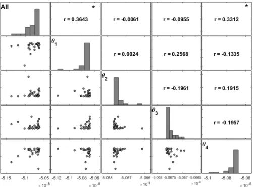
Figure 9.Matrix plot of the maximum transverse displacement(wmax)considering different sets of uncertain stacking angles for Case 1.c (a/h = 20, [0/90]2).

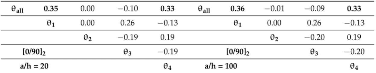
Table 6.Correlation coefficients obtained with uncertain stacking angles for Case 1.c (left) and Case 2.c (right).

θ_all 0.35 0.00 −0.10 0.33 θ_all 0.36 −0.01 −0.09 0.33

θ1 0.00 0.26 −0.13 θ1 0.00 0.26 −0.13

θ2 −0.19 0.19 θ2 −0.20 0.19

[0/90]2 θ3 −0.19 [0/90]2 θ3 −0.20

a/h = 20 θ4 a/h = 100 θ4

The results in Tables5and6are similar, despite the difference between stacking sequences. Note that the correlation coefficient for θ1is higher in these cases, reaching values similar to those for θ4

(Table6). On the other hand, Table5shows that the correlation for [0/90]Spresents higher values for

all stacking angles, with the value for θ4remaining the highest.

3.3. Uncertainty in the Layer Thickness

In the present work, the variability on the maximum deflection due to uncertain ply thicknesses was also analysed. Figure10shows the same type of matrix plot but for Case 3.a.

Matrix plots were constructed and analysed for all of the studied cases. However, for the sake of simplicity, Tables7–9summarise the results obtained.

The correlation coefficients between samples for maximum transverse displacement for almost all case studies are dominated by the uncertain properties of the fourth ply (Tables7–9). A correspondence can be observed with the results presented in the previous sections, although for the ply thickness higher values are obtained for the correlation coefficients.

Comparing the cases with uncertain stacking angles (Cases 1 and 2) and those with uncertain ply thicknesses (Cases 3 and 4) for different aspect ratios, there is greater consistency in the distributions of the maximum transverse displacement for Cases 3 and 4 (Figures10–12), which are almost symmetric. On the other hand, for Cases 1 and 2, there are significant changes in the aspect ratios and stacking sequences (Figures6–9).

(13)

J. Compos. Sci. 2018, 2, 6 13 of 17

In the cases with uncertain ply thicknesses, the correlation coefficients for the thickness of the fourth ply (h4) overcome all the others with values near 1.0 (Figures11and12), with the exception of Cases 3.b and 4.b.

From Tables7–9, it is possible to conclude that the fourth ply is by far the most significant parameter.

Table 7.Correlation coefficients obtained with uncertain ply thicknesses for Case 3.a (left) and Case 4.a (right).

h_all 0.10 0.17 0.24 0.97 h_all 0.10 0.17 0.24 0.97

h1 −0.01 −0.01 0.02 h1 −0.01 −0.01 0.02

h₂ 0.04 0.09 h₂ 0.04 0.10

[0]4 h3 0.02 [0]4 h3 0.02

a/h = 20 h₄ a/h = 100 h₄

Table 8.Correlation coefficients obtained with uncertain ply thicknesses for Case 3.b (left) and Case 4.b (right).

h_all 0.06 0.25 0.45 0.88 h_all 0.06 0.26 0.45 0.88

h1 −0.02 0.00 0.02 h1 −0.02 0.00 0.02

h2 0.05 0.10 h2 0.05 0.10

[0/90]S h3 0.01 [0/90]S h3 0.01

a/h = 20 h4 a/h = 100 h4

Table 9.Correlation coefficients obtained with uncertain ply thicknesses for Case 3.c (left) and Case 4.c (right).

hall 0.10 0.18 0.24 0.97 hall 0.09 0.18 0.22 0.97

h1 −0.01 0.00 0.02 h1 −0.01 0.00 0.02

h2 0.05 0.10 h2 0.05 0.10

[0/90]2 h3 0.02 [0/90]2 h3 0.02

a/h = 20 h4 a/h = 100 h4

In the cases with uncertain ply thicknesses, the correlation coefficients for the thickness of the fourth ply (h4) overcome all the others with values near 1.0 (Figures 11 and 12), with the exception of Cases 3.b and 4.b.

From Tables 7–9, it is possible to conclude that the fourth ply is by far the most significant parameter.

Table 7. Correlation coefficients obtained with uncertain ply thicknesses for Case 3.a (left) and Case 4.a (right). hall 0.10 0.17 0.24 0.97 hall 0.10 0.17 0.24 0.97 h1 −0.01 −0.01 0.02 h1 −0.01 −0.01 0.02 h2 0.04 0.09 h2 0.04 0.10 [0]4 h3 0.02 [0]4 h3 0.02 / = h4 / = h4

Table 8. Correlation coefficients obtained with uncertain ply thicknesses for Case 3.b (left) and Case 4.b (right). hall 0.06 0.25 0.45 0.88 hall 0.06 0.26 0.45 0.88 h1 −0.02 0.00 0.02 h1 −0.02 0.00 0.02 h2 0.05 0.10 h2 0.05 0.10 [0/90]S h3 0.01 [0/90]S h3 0.01 / = h4 / = h4

Table 9. Correlation coefficients obtained with uncertain ply thicknesses for Case 3.c (left) and Case 4.c (right). hall 0.10 0.18 0.24 0.97 hall 0.09 0.18 0.22 0.97 h1 −0.01 0.00 0.02 h1 −0.01 0.00 0.02 h2 0.05 0.10 h2 0.05 0.10 [0/90]2 h3 0.02 [0/90]2 h3 0.02 / = h4 / = h4

Figure 10. Matrix plot of the ply thicknesses (h1–h4) and the resulting maximum deflection (w ) and fundamental frequency (f ) for Case 3.a (a/h = 20, [0]4).

Figure 10.Matrix plot of the ply thicknesses (h1–h4) and the resulting maximum deflection(wmax) and fundamental frequency (f1) for Case 3.a (a/h = 20, [0]4).

(14)

Figure 11. Matrix plot of the maximum transverse displacement (w ) considering different sets of uncertain ply thicknesses for Case 3.c (a/h = 20, [0/90]2).

Figure 12. Matrix plot of the maximum transverse displacement (w ) considering different sets of uncertain ply thicknesses for Case 4.b (a/h = 100, [0/90]S).

3.4. Regression Models

In the previous case studies, we assessed the correlation of the material and geometrical parameters, assuming different uncertain sets. From those studies, it is already possible to conclude that some parameters are more significant for the plate responses.

The present study intended to build probabilistic models to represent the unidirectional composite plate response, both in the case of its maximum transverse deflection (w ) and in the case of its fundamental frequency (f ). To this purpose, a multivariable linear regression approach (Section 2.5) has been considered. According to this methodology, the models predicting those two responses were initially written as:

Figure 11.Matrix plot of the maximum transverse displacement(wmax)considering different sets of uncertain ply thicknesses for Case 3.c (a/h = 20, [0/90]2).

Figure 11. Matrix plot of the maximum transverse displacement (w ) considering different sets of uncertain ply thicknesses for Case 3.c (a/h = 20, [0/90]2).

Figure 12. Matrix plot of the maximum transverse displacement (w ) considering different sets of uncertain ply thicknesses for Case 4.b (a/h = 100, [0/90]S).

3.4. Regression Models

The present study intended to build probabilistic models to represent the unidirectional composite plate response, both in the case of its maximum transverse deflection (w ) and in the case of its fundamental frequency (f ). To this purpose, a multivariable linear regression approach (Section 2.5) has been considered. According to this methodology, the models predicting those two responses were initially written as:

Figure 12.Matrix plot of the maximum transverse displacement(wmax)considering different sets of uncertain ply thicknesses for Case 4.b (a/h = 100, [0/90]S).

3.4. Regression Models

The present study intended to build probabilistic models to represent the unidirectional composite plate response, both in the case of its maximum transverse deflection (wmax) and in the case of its

fundamental frequency (f1). To this purpose, a multivariable linear regression approach (Section2.5)

has been considered. According to this methodology, the models predicting those two responses were initially written as:

wmax=β0+β1E11+β2E22+β3ν12+β4G12+β5G13+β6G23+β7h+ε

f1=β0+β1E11+β2E22+β3ν12+β4G12+β5G13+β6G23+β7h+β8ρ+ε

(15)

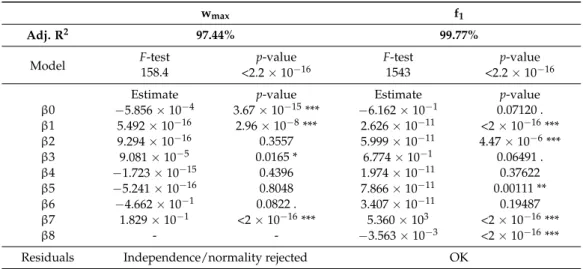
The results obtained for the different regression coefficients βiare summarized in Table10. It is

important to mention that a set of significance codes were used to classify the significance of each regression coefficient based on the p-value of the t-test.

From Table10, it is possible to conclude on the very high values of the adjusted R2. However, concerning the maximum transverse deflection regression model, the hypothesis of independence and normality of the residuals has been rejected, which does not happen in the case of the model for the fundamental frequency where all of the model assumptions have been verified.

Concerning the regression model for the maximum deflection, we conclude that the most significant parameters are the longitudinal elasticity modulus(E11)and the plate thickness h. Poisson’s

ratio(ν₁₂)and the shear modulus G23are the next two in terms of significance.

For the fundamental frequency, all of the parameters are significant except the shear moduli G12

and G23. However, we consider the regression model for the fundamental frequency validated, even

with some nonsignificant variables.

Table 10.Multivariable linear regression models—initial case summaries.

wmax f1

Adj. R2 97.44% 99.77%

Model F-test p-value F-test p-value

158.4 <2.2 × 10−16 ₁₅₄₃ _{<2.2 × 10}−16

Estimate p-value Estimate p-value

β0 −5.856 × 10−4 _{3.67 × 10}−15_*** _{−6.162 × 10}−1 _{0.07120 .} β1 5.492 × 10−16 _{2.96 × 10}−8_*** _{2.626 × 10}−11 _{<2 × 10}−16_*** β2 9.294 × 10−16 _0.3557 _{5.999 × 10}−11 _{4.47 × 10}−6_*** β3 9.081 × 10−5 0.0165 * 6.774 × 10−1 0.06491 . β4 −1.723 × 10−15 _0.4396 _{1.974 × 10}−11 _0.37622 β5 −5.241 × 10−16 _0.8048 _{7.866 × 10}−11 _{0.00111 **} β6 −4.662 × 10−1 _{0.0822 .} _{3.407 × 10}−11 _0.19487 β7 1.829 × 10−1 <2 × 10−16*** 5.360 × 103 <2 × 10−16*** β8 - - −3.563 × 10−3 _{<2 × 10}−16_***

Residuals Independence/normality rejected OK

Significance codes: 0 “***” 0.001 “**” 0.01 “*” 0.05 “.” 0.1 “ ” 1.

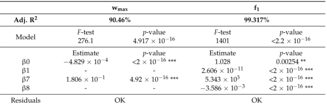
Therefore, in a second stage of this study we considered alternative models considering only the previous most significant parameters in both cases. After a forward selection process, the following simplified models were obtained:

wmax=β0+β7h+ε

f1= β0+β1E11+β7h+β8ρ+ε

(7)

The results for these final models are presented in Table11.

It is worth mentioning that there was no need for an alternative model in the case of the fundamental frequency, although this was considered.

From the results in Table11, it is possible to say that the simplified models (Equation (7)) present high values of adjusted R2, and in both cases the residuals assumptions are verified. Therefore, these simplified models are validated. Moreover, it can be observed that in the case of the maximum deflection model, by considering only the thickness, we attain a model that explains 90.46% of the plate deflection variability. For the simplified fundamental frequency model, a very high explanation (99.317%) is obtained, continuing to observe the residuals assumptions.

It is relevant to note that an intermediate simplified model for the maximum deflection can be given by:

(16)

where E11 is included. However, in this case, the residuals problems persisted, although the value

of the adjusted R2is 97.58 %. The normality of the residuals was improved when compared to the model in Equation (7), but the residuals independency was not guaranteed as observed in Figure13. Considering this, it is not possible to accept the corresponding multivariable linear regression model.

Table 11.Multivariable linear regression models—simplified case summaries.

wmax f1

Adj. R2 90.46% 99.317%

Model F-test_276.1 _{4.917 × 10}p-value−16 F-test₁₄₀₁ _{<2.2 × 10}p-value−16

Estimate p-value Estimate p-value

β0 −4.829 × 10−4 _{<2 × 10}−16_*** _1.028 _{0.00254 **} β1 - - 2.606 × 10−11 <2 × 10−16*** β7 1.806 × 10−1 4.92 × 10−16*** 5.343 × 103 <2 × 10−16*** β8 - - −3.586 × 10−3 _{<2 × 10}−16_*** Residuals OK OK Significance codes: 0 “***” 0.001 “**” 0.01 “*” 0.05 “.” 0.1 “ ” 1.

Table 11. Multivariable linear regression models—simplified case summaries.

Adj. 90.46% 99.317%

Model F-test p-value F-test p-value

276.1 4.917 × 10−16 ₁₄₀₁ _{<2.2 × 10}−16

Estimate p-value Estimate p-value

β0 −4.829 × 10−4 _{<2 × 10}−16_*** _1.028 _{0.00254 **} β1 - - 2.606 × 10−11 _{<2 × 10}−16_*** β7 1.806 × 10−1 _{4.92 × 10}−16_*** _{5.343 × 10}3 _{<2 × 10}−16_*** β8 - - −3.586 × 10−3 _{<2 × 10}−16_*** Residuals OK OK Significance codes: 0 “***” 0.001 “**” 0.01 “*” 0.05 “.” 0.1 “ ” 1.

It is relevant to note that an intermediate simplified model for the maximum deflection can be given by:

w = β + β E + β h + ε (8)

where E is included. However, in this case, the residuals problems persisted, although the value of the adjusted R is 97.58 %. The normality of the residuals was improved when compared to the model in Equation (7), but the residuals independency was not guaranteed as observed in Figure 13. Considering this, it is not possible to accept the corresponding multivariable linear regression model.

Figure 13. Residuals of the regression model for w (Equation (8)).

4. Conclusions

This work presents a study on the uncertainty propagation of the geometrical and material parameters on the mechanical response of carbon fibre-reinforced composite laminate. The simulation of the uncertain modelling parameters was carried out by considering a random multivariate normal distribution.

The significance of each material and geometrical parameters on the simulated linear static and free vibration response of a certain composite structure was assessed and, therefore, the characterization of the response variability was analysed and conclusions were drawn.

From the obtained results, it is possible to conclude that the variability of the maximum transverse deflection and fundamental frequency is more sensitive to laminate thickness than to other parameters. The longitudinal elasticity modulus (E ) appears as the second most significant parameter and the density is the next, when considering the laminate fundamental frequency.

It is also important to summarize the greater sensitivity of the simulated static response to changes on the geometrical parameters of external layers, namely the upper one. Additional simulations were carried out for a larger sample size, confirming the presented conclusions, although this topic should be addressed in more detail in future studies.

The multivariable linear regression analysis confirms the conclusions of the presented correlation analysis in what concerns the influence of the material properties and the global thickness of the laminate. Valid multivariable linear regression models were obtained for the response

Figure 13.Residuals of the regression model for wmax(Equation (8)).

4. Conclusions

This work presents a study on the uncertainty propagation of the geometrical and material parameters on the mechanical response of carbon fibre-reinforced composite laminate. The simulation of the uncertain modelling parameters was carried out by considering a random multivariate normal distribution.

The significance of each material and geometrical parameters on the simulated linear static and free vibration response of a certain composite structure was assessed and, therefore, the characterization of the response variability was analysed and conclusions were drawn.

From the obtained results, it is possible to conclude that the variability of the maximum transverse deflection and fundamental frequency is more sensitive to laminate thickness than to other parameters. The longitudinal elasticity modulus(E11)appears as the second most significant parameter and the

density is the next, when considering the laminate fundamental frequency.

It is also important to summarize the greater sensitivity of the simulated static response to changes on the geometrical parameters of external layers, namely the upper one. Additional simulations were carried out for a larger sample size, confirming the presented conclusions, although this topic should be addressed in more detail in future studies.

The multivariable linear regression analysis confirms the conclusions of the presented correlation analysis in what concerns the influence of the material properties and the global thickness of the laminate. Valid multivariable linear regression models were obtained for the response variables, allowing for the identification of the most important parameters regarding the description of the response variability.

(17)

As a final global conclusion, it is considered that under the present assumptions, this methodological study provides an effective tool to characterize the relative influence of each modelling parameter on the explanation of the variability of the mechanical response predictions.

Acknowledgments:The authors wish to acknowledge the financial support of Project IPL/2016/CompDrill/ISEL and the support of Fundação para a Ciência e a Tecnologia through Project LAETA-UID/EMS/50022/2013, Project UNIDEMI-Pest-OE/EME/UI0667/2014 and Project CEMAPRE-UID/Multi/00491/2013.

Author Contributions:All authors contributed to the design and implementation of the research, to the analysis of the results and to the writing of the manuscript.

Conflicts of Interest:The authors declare no conflict of interest. References

1. Schemme, M. LFT—Development status and perspectives. Reinf. Plast. 2008, 52, 32–34. [CrossRef]

2. State of the Composites Industry Report for 2017. Available online:http://compositesmanufacturingmagazine.

com/2017/01/composites-industry-report-2017(accessed on 1 November 2017).

3. Prashanth, S.; Subbaya, K.M.; Nithin, K.; Sachhidananda, S. Fiber Reinforced Composites—A Review. J. Mater. Sci. Eng. 2017, 6, 1–6.

4. Mesogitis, T.S.; Skordos, A.A.; Long, A.C. Uncertainty in the manufacturing of fibrous thermosetting composites: A review. Compos. A Appl. Sci. Manuf. 2014, 57, 67–75. [CrossRef]

5. Noor, A.K.; Starnes, J.H., Jr.; Peters, J.M. Uncertainty analysis of composite structures. Comput. Methods Appl. Mech. Eng. 2000, 185, 413–432. [CrossRef]

6. António, C.A.C.; Hoffbauer, L.N. Uncertainty assessment approach for composite structures based on global sensitivity indices. Compos. Struct. 2013, 99, 202–212. [CrossRef]

7. Teimouri, H.; Milani, A.S.; Seethaler, R.; Heidarzadeh, A. On the Impact of Manufacturing Uncertainty in Structural Health Monitoring of Composite Structures: A Signal to Noise Weighted Neural Network Process. Open J. Compos. Mater. 2016, 6, 28–39. [CrossRef]

8. Mukherjee, S.; Ganguli, R.; Gopalakrishnan, S.; Cot, L.D.; Bes, C. Ply Level Uncertainty Effects on Failure of Composite Structures. Le Cam, Vincent and Mevel, Laurent and Schoefs, Franck. In Proceedings of the EWSHM—7th European Workshop on Structural Health Monitoring, Nantes, France, 8–11 July 2014. 9. Hohe, J.; Beckmann, C.; Paul, H. Modeling of uncertainties in long fiber reinforced thermoplastics. Mater. Des.

2015, 66, 390–399. [CrossRef]

10. Carvalho, A.; Silva, T.; Loja, M.A.R.; Damásio, F.R. Assessing the influence of material and geometrical uncertainty on the mechanical behavior of functionally graded material plates. Mech. Adv. Mater. Struct.

2017, 24, 417–426. [CrossRef]

11. Reddy, J.N. Mechanics of Laminated Composite Plates; CRC Press: Boca Raton, FL, USA, 1997.

12. Loja, M.A.R.; Barbosa, J.I.; Mota Soares, C.M. Analysis of Sandwich Beam Structures Using Kriging Based Higher Order Models. Compos. Struct. 2015, 119, 99–106. [CrossRef]

13. Loja, M.A.R.; Barbosa, J.I.; Mota Soares, C.M. Dynamic Behaviour of Soft Core Sandwich Structures using Kriging-Based Layerwise Models. Compos. Struct. 2015, 134, 883–894. [CrossRef]

14. Loja, M.A.R.; Barbosa, J.I.; Mota Soares, C.M. Dynamic Instability of Variable Stiffness Composite Plates. Compos. Struct. 2017, 182, 402–411. [CrossRef]

15. Iman, R.L.; Conover, W.J. A Distribution-Free Approach to Inducing Rank Correlation Among Input Variables. Commun. Stat. B 1982, 11, 311–334. [CrossRef]

article distributed under the terms and conditions of the Creative Commons Attribution (CC BY) license (http://creativecommons.org/licenses/by/4.0/).