UNIVERSIDADE DE ÉVORA
DEPARTAMENTO DE ECONOMIA
DOCUMENTO DE TRABALHO Nº 2005/19
November
Immunization Using a Parametric Model of the Term
Structure
Jorge Miguel Ventura Bravo *
Universidade de Évora, Departamento de Economia
Carlos Manuel Pereira da Silva
ISEG - School of Economics and Management, Technical University of Lisbon This Draft: May 2005
* We acknowledge comments from Professor Carlos Braumann and from participants at the 8th International Congress on Insurance: Mathematics & Economics, Rome June 2004 and at the 3rd Portuguese Finance Network Conference, Lisbon, July 2004.
UNIVERSIDADE DE ÉVORA DEPARTAMENTO DE ECONOMIA
Largo dos Colegiais, 2 – 7000-803 Évora – Portugal Tel.: +351 266 740 894 Fax: +351 266 742 494
Abstract/Resumo:
In this paper, we develop a new immunization model based on a parametric specification of the term structure of interest rates. The model extends traditional duration analysis to account for both parallel and non-parallel term structure shifts that have an economic meaning. Contrary to most interest rate risk models, we analyse both first-order and second-order conditions for bond portfolio immunization and conclude that the key to successful protection will be to build up a bond portfolio such that the gradient of its future value is zero, and such that its Hessian matrix is positive semidefinite. In addition, we provide explicit formulae for new parametric interest rate risk measures and present alternative approaches to implement the immunization strategy. Furthermore, we provide useful expressions for the sensitivity of interest rate risk measures to changes in term structure shape parameters.
Palavras-chave/Keyword: Immunization; duration; parametric model; interest rate risk Classificação JEL/JEL Classification: E43, G11
1
Introduction
Immunization, which may be de…ned as the protection of the nominal value of a portfolio (or the net value of a …rm) against changes in the term structure of interest rates, is a well-known area of portfolio management. Immunization allows the setting up and management of a bond portfolio in such a way that this portfolio reaches a predetermined goal. This goal can either be to guarantee a set of future payments, to obtain a certain rate of return for the investment or, in certain cases, to replicate the performance of a bond market index. Immunization models (also known as interest-rate risk or duration models) control risk through duration and convexity measures, which capture the sensitivity of bond returns to changes in one or more interest rate risk factors.
The traditional approach to immunization employs duration measures derived analytically from prior assumptions regarding speci…c changes in the term structure of interest rates.1 Un-fortunately, in this case the e¤ectiveness of the strategy is compromised, since the investment is protected only against the particular type of interest rate change assumed. Fong and Vasicek (1983, 1984) developed the M-Squared model in order to minimize the immunization risk due to non-parallel (slope) shifts in the term structure of interest rates. The authors show in particular that by setting the duration of a bond portfolio equal to its planning horizon and by minimizing a quadratic cash ‡ow dispersion measure, the immunization risk due to adverse term structure shifts can be reduced.2 More recently, new immunization risk (dispersion) measures were proposed by
Nawalkha and Chambers (1996), Balbás and Ibáñez (1998) and Balbás et al.(2002).
In recent years researchers have redirected their attention towards the development of alterna-tive formulations which try to capture more e¤ecalterna-tively the interest rate risk faced by …xed-income portfolios, without relying on any particular assumptions as to the type of stochastic process which governs interest rate movements. A popular approach is to assume that interest rate changes can be accurately described by shifts in the level of a limited number of segments (vertices or yield
1For example, the duration measure developed by Fisher and Weil (1971) assumes a parallel and instantaneous shift in the term structure of interest rates. Non-parallel shifts were proposed by Bierwag (1977), Khang (1979) and Babbel (1983) or, in an equilibrium setting, by Cox et al. (1979), Ingersoll et al. (1978), Brennan and Schwartz (1983), Nelson and Schaefer (1983) and Wu (2000), among others.
2Nawalkha and Chambers (1997) and Nawalkha, Soto and Zhang (2003) derive a multiple-factor extension to the M-Squared model termed M-Vector Model.
curve drivers) into which the term structure is subdivided, generalizing then the concepts of dura-tion and convexity to a multivariate context by considering the portfolio’s joint exposure to these key rates. Speci…cally, we refer to the directional duration and to the partial duration models of Reitano (1990, 1991a, 1991b, 1992), to the key-rate duration model of Ho (1992) and to the reshaping duration model suggested by Kla¤ky et al.. (1992). In these models, the direction of interest rate shifts can be set on an a priori basis, or can be based on real data. In the latter case, the historical movements in the term structure of interest rates are used to identify a limited number of state variables, observable or not, which govern the yield curve.3
An alternative line of attack to the problem of immunization involves the use of parametric duration models. In this kind of formulation, which has its roots in the work of Cooper (1977), all that is assumed is that at each moment in time, the term structure of interest rates adheres to a particular functional form, which expresses itself as a function of time and a limited number of shape parameters. In this line of thought, provided that the mathematical function …ts most yield curves accurately all interest rate movements can be expressed in terms of changes in one or more shape parameters that characterize this function. In other words, it is apparent that in this kind of models, the interest rate risk uncertainty is re‡ected by the unknown nature of future parameter values. Di¤erentiating the bond price with respect to each shape parameter we obtain a vector of parametric interest rate risk measures. Choosing a particular functional form obviously involves some pricing errors. The di¤erence is that in this case the errors can be quanti…ed and controlled systematically, as long as we are able to choose the appropriate speci…cation for the yield curve, in which by ’appropriate’ we mean the speci…cation that minimizes immunization risk.
Since the work of Cooper, there has been little research in this area. Garbade (1985), Chambers et al. (1988) and Prisman and Shores (1988) assume that a polynomial may be used to …t the term structure of interest rates as a …rst step to derive a vector of interest rate risk measures -termed a duration vector -, in which each element basically corresponds to the moment of order k of a bond4. Although simple, the use of polynomial functions to estimate the yield curve has
been subject to great criticism, since it can lead to forward curves that exhibit undesirable (and
3See, for example, Gultekin and Rogalski (1984), Elton et al. (1990), Garbade (1986), Litterman and Scheinkman (1991), Knez et al. (1994), D’Ecclesia and Zenios (1994), Barber and Copper (1996) and Bravo and Silva (2005).
4The moment of order k of a bond is de…ned as the weighted average of the kth power of its times of payments, the weights being the shares of the bond’s cash ‡ows in present value in the bond’s present value. Chambers et al.
unrealistic) properties for long maturities, namely high instability. In Willner (1996), the actual yield curve risk exposure of a bond portfolio is decomposed using the Nelson and Siegel (1987) parametrization of the yield curve, a mathematical function that expresses interest rates in terms of four parameters and is compatible with standard increasing, decreasing, ‡at and inverted yield curve shapes.
In this paper, we develop a new immunization model based on the Svensson (1994) speci…cation of the yield curve. The model is parametric by nature, i.e., the interest rate risk factors correspond to the parameters of the mathematical function used to represent the yield curve. Furthermore it adopts a multivariate setting, being compatible with both parallel and non-parallel term structure shifts. Since we do not impose any previous assumptions as to the way the yield curve changes, the model is applicable in virtually all yield curve environments. In addition, the model is intuitive and relatively easy to apply.
This paper is related to Willner (1996), but there are some important di¤erences. First, we adopt Svensson’s parametrization instead of Nelson and Siegel’s mathematical function. As shown by Svensson (1994), the extended form allows more ‡exibility in the yield curve estimation, in particular in the short-term end of the yield curve. In addition, the model assumes that every movement in the term structure of interest rates can be approximated by changes in a small number of factors and that these factors can be directly interpreted as representing parallel, slope and curvature shifts in the yield curve. Second, contrary to Willner and most interest rate risk models, we formally analyze both …rst-order and second-order conditions for bond portfolio im-munization, emphasizing that the key to successful immunization will be to build up a portfolio such that the gradient of its future value is zero, and such that its Hessian matrix is positive semide…nite. Moreover, we provide explicit formulae for new parametric interest rate risk mea-sures and present alternative approaches to implement the immunization strategy. Finally, we extend previous analysis on the sensitivity of a bond’s duration to changes in the yield to maturity by developing useful expressions for the sensitivity of parametric interest rate risk measures to changes in term structure shape parameters.
The paper is organized as follows. In Section 2, we brie‡y characterize Svensson’s speci…cation of the yield curve and theoretically justify its use in the context of the immunization problem.
(1988) perform immunization tests for the U.S. market over single-and multi-period horizons and conclude that the improvement in the immunization performance is considerable when at least four interest rate risk measures are added.
In Section 3, we introduce the concepts of parametric duration and parametric convexity and formally derive …rst-order and second-order conditions for immunization. We show that it is impossible to achieve immunization simply by meeting …rst-order conditions and that second-order conditions must be addressed appropriately. In Section 4, we provide simple expressions for the sensitivity of parametric interest rate risk measures to changes in term structure shape parameters. Section 5 summarizes the main conclusions of the paper.
2
Term Structure Speci…cation
The Svensson (1994) model is a parametric model which assumes that the instantaneous forward rate, f (t; a): f (t; a) = a0+ a1 exp t a4 + a2 t a4 exp t a4 + a3 t a5 exp t a5 ; (1)
is a function of both the time to maturity t and a (line) vector of parameters a = (a0; a1; a2; a3; a4; a5)
to be estimated, with (a0; a4; a5) > 0. To increase the ‡exibility of the curves and to improve
the …t, Svensson extended Nelson and Siegel’s functional form by adding a potential extra hump in the forward curve. It is well known that the Nelson-Siegel method admits the existence of only one extremum and one point of in‡ection in the concavity. This means that when there are disturbances in the money market that lead to curves with two local extrema, the …t in the short segment of the yield curve turns out to be very poor. Given its higher adjustment capacity, the Svensson model has proven to be more adequate in estimating the term structure of interest rates and it is widely used by practitioners and major central banks.5
The parameters in the forward rate function are estimated by solving a non-linear optimization procedure to data observed on a trade day, which consists of minimizing the sum of squared yield (or price) deviations between observed and theoretical yields (or prices) as estimated with the model. The optimization problem can be solved using either a grid search procedure or a partial estimation technique6. In most practical applications, …tting was found to be relatively insensitive
5The Bank of International Settlements (1999) notes that ten Central Banks (of twelve surveyed) routinely use either the Nelson and Siegel (1987) and/or the Svensson (1994) model as their primary method for analyzing the yield curve. See Bravo (2001), Barrett et al. (1995), Diebold and Li (2003) for other uses of the NS model.
6For more details on the estimation process see, for example, Nelson and Siegel (1987), BIS (1999) and Bolder and Stréliski (1999).
to changes in parameters a4 and a5 (e.g. Barrett et al., 1995, Willner, 1996 and Diebold and Li,
2003). Without loss of generality, we will follow standard practise and assume at any stage that these parameters are …xed at prespeci…ed values. Note also that by setting a3 equal to zero in
(1), we obtain the Nelson and Siegel forward rate function.
Regardless of their popularity, the Nelson-Siegel-Svensson family of curves has been criticized because of two theoretical shortcomings. The …rst, pointed out by Björk and Christensen (1999) and Filipovic (1999, 2000), is that models …tted sequentially to cross-sectional data are not inter-temporally consistent with the dynamics of a given interest rate model. Björk and Christensen (1999) prove, for instance, that the Nelson-Siegel family of curves is inconsistent with the Ho-Lee interest rate model and with the Hull-White extension of the Vasicek model. This feature weakens the validity of the model for applications that involve a time-series context. It can be shown, however, that a simple manifold expansion (i.e. the addition of appropriate functions of maturity) is su¢ cient to make the Nelson and Siegel model consistent with given interest rate models, particularly with the generalized Vasicek short rate model.7 Nonetheless, these adjustments impose additional constraints on the estimation of the models to cross-sectional data, thus leading to a non-trivial deterioration of the …tting performance when compared with that provided by the Nelson-Siegel-Svensson family of curves. On the other hand, it is not obvious to us that the use of arbitrage-free models is necessary or desirable for accomplishing good immunization performance. Indeed, if the theoretical superiority of equilibrium term structure models is unquestionable, when compared to traditional immunizing duration models, the truth is that a number of papers, such as Ingersoll (1983), Nelson and Schaefer (1983) and Brennan and Schwartz (1983), have shown that their immunization performance is rather similar. In addition, Brandt and Yaron (2003) prove that typical no-arbitrage models are actually time-inconsistent because their parameters are assumed constant for pricing purposes, even though the parameters change each time the model is recalibrated to data observed on a given date. Moreover, recent studies (e.g. Du¢ e, 2002 and Dai and Singleton, 2002) have shown that a¢ ne no-arbitrage models can produce poor forecasts.
The second theoretical shortcoming is that these models apparently lack a fundamental eco-nomic foundation, which leads researchers to be cautious when interpreting the parameters in conjunction with economic variables, and may explain why their use has been limited to cross-sectional applications, namely, yield-curve …tting and interest rate risk management. An
ception is given by Diebold and Li (2003), who use variations on the Nelson-Siegel framework to model the entire yield curve on an inter-temporally basis as a three-dimensional parameter evolving dynamically.8 The authors prove, …rst, that the model is consistent with standard
styl-ized facts regarding the yield curve and, second, that the three-time varying parameters may be roughly interpreted as factors corresponding to level, slope and curvature, a result consistent with previous studies on this subject.9
From (1), the continuously compounded zero-coupon curve r(t; a) can be derived, noting that r(t; a) = 1t R0tf (t; a)dt: r(t; a) = a0+ a1 a4 t 1 e t a4 + a2a4 t 1 e t a4 1 + t a4 + a3 a5 t 1 e t a5 1 + t a5 ; (2) whereas the discount function d(t; a) is de…ned as:
d(t; a) = exp [ r(t; a)t] : (3)
Each parameter in (1) has a particular impact on the shape of the forward rate curve. Para-meter a0, which represents the asymptotic value of f (t; a) (i.e., limt!1f (t; a) = a0), can actually
be regarded as a long-term (consol) interest rate. Parameter a1 de…nes the speed with which
the curve tends towards its long-term value. The yield curve will be upward sloping if a1 < 0
and downward-sloping if a1 > 0. The higher the absolute value of a1 the steeper the yield curve.
Notice also that the sum of a0 and a1 corresponds to the instantaneous forward rate with an
in…n-itesimal maturity (limt!0f (t; a) = a0+ a1), i.e., it de…nes the intercept of the curve. Parameters
a2 and a3 have similar signi…cance and in‡uence the shape of the yield curve. They determine
the magnitude and the direction of the …rst and second humps, respectively. For example, if a2
is positive, a hump will occur at a4 whereas, if a2 is negative, a U-shape value will emerge at a4.
Parameters a4 and a5, which are always positive, have similar roles and de…ne the position of the
…rst and second humps, respectively.
The Svensson model is very intuitive since parameters a0, a1, a2 and a3 (the interest rate
factors) can directly be linked to parallel displacements, slope changes and curvature shifts in the
8See also Krippner (2005b).
9See, for instance, Litterman and Scheinkman (1991), Barber and Copper (1996), Knez et al. (1994), D’Ecclesia and Zenios (1994) and Bravo and Silva (2005).
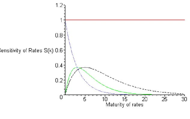
yield curve, given that scale coe¢ cients are …xed. To perceive this behavior, Figure 1 displays the sensitivity Sk= @f (t;a)@a
k of forward rates to each parameter ak, for k = 0; :::; 3.
[Insert Figure 1, about here]
As can be seen, the sensitivity of forward rates with respect to the consol rate is constant across the whole maturity spectrum, which means that it can actually be regarded as a level factor. In other words, the level factor S0 fundamentally represents a parallel displacement in
the term structure of interest rates. The sensitivity of interest rates to changes in parameter a1
shows a descending shape, …rst larger for shorter maturities, then declining exponentially toward zero as maturity increases. In this sense, factor S1 is a slope factor and represents changes in the
steepness of the yield curve. Finally, factors S2 and S3 have di¤erent impacts on intermediate
rates as opposed to extreme maturities (short and long), reaching a maximum on those points (a4
and a5, respectively) where the yield curve has humps. Hence, these factors may be interpreted
as curvature factors. In brief, the Svensson model assumes that: (i) every movement in the term structure of interest rates can be approximated by changes in only four factors; (ii) these factors take familiar shapes, that is parallel shifts, changes in steepness, and changes in the curvature of the yield curve.
3
Constructing Immunized Portfolios
Consider an investor who has a position in a number L of default-free bonds. Let clt denote the
nominal cash ‡ow (in monetary units) received from bond l (l = 1; :::; L) at time t (t = 1; :::; N ). Let t = 0 be the current date, and H a known, …nite investment horizon, measured in years. Assuming that the initial term structure is known and described by the parametric function (2), which assigns a spot rate to each payment date t, the present value of bond l, Bl
0(a), is given by:
B0l(a) = N X t=1 cltexp [ r(t; a)t] = = N X t=1 clte a0+a1a4t 1 e t a4 +a2a4t 1 e t a4 1+ t a4 +a3a5t 1 e t a5 1+ t a5 t; (4)
where we have stressed the functional relationship between the bond price Bl(a) and the initial
vector a = (a0; a1; a2; a3; a4; a5) T
of parameters of the forward rate function. Let nl represent the
number of type l bonds in the portfolio. In this case, the present value (at time 0) of this bond portfolio, P0(a), is given by:
P0(a) = L X l=1 nlB0l(a) = L X l=1 N X t=1 nlcltexp [ r(t; a)t] = = L X l=1 N X t=1 nlclte a0+a1a4t 1 e t a4 +a2a4t 1 e t a4 1+ t a4 +a3a5t 1 e t a5 1+ t a5 t (5)
For simplicity of exposition, consider now that the investor is interested only in his wealth position at some future time H (where H might represent, for example, the due date on a single liability payment). The value of this portfolio at time H, under the expectations hypothesis of the term structure assuming no change in the yield curve, PH(a), will be:
PH(a) = P0(a) exp [r(H; a)H] =
= " L X l=1 N X t=1 nlcltexp [ r(t; a)t] # exp [r(H; a)H] (6)
Suppose now that at time , immediately after the investor purchased the portfolio, the spot rate function has undergone a variation, which may be viewed here as a vector dA of multiple random shifts and represent both parallel and nonparallel shifts, such that the new term structure, represented again by Svensson’s model, is r (t; A) = r(t; a + dA ):
r (t; A) = A0+ A1 A4 t 1 e t A4 + A2A4 t 1 e t A4 1 + t A4 +A3 A5 t 1 e t A5 1 + t A5 ; (7) where A = (A0; :::; A5) T
denotes the new vector of coe¢ cients of the spot rate function estimated at time . The new terminal value of the portfolio, PH(A), keeps the same form as above, except
that vector A now replaces the initial vector of parameters a:
PH(A) = " L X l=1 N X t=1 nlcltexp [ r(t; A)t] # exp [r(H; A)H] (8)
The traditional de…nition of immunization (e.g. Fisher and Weil, 1971) for the case of a single liability establishes that a portfolio of default-free bonds is said to be immunized against any type of interest rate shifts if its accumulated value at the end of the planning horizon is at least as great as the target value, where the target value is de…ned as the portfolio value at the horizon date under the scenario of no change in the spot (and forward) rates. Stated more formally, by immunization we mean selection of a bond portfolio such that the actual future value of the income stream PH(A)at time H will exceed the initially expected value PH(a), i.e., PH(A) PH(a) (or
equivalently, PH = PH(A) PH(a) 0), if the interest rates r(t; A) shift to their new value
r (t; A).
Under the assumption that interest rates only change by a parallel shift, the main conclusion of Fisher and Weil was that immunization is achieved when the duration of the portfolio is set equal to the length of the investment horizon. The assumption that interest rates can change only by a parallel shift is very restrictive and can carry serious risks. In this paper we o¤er a more generalized approach to immunization by deriving the conditions under which the investment is protected against both parallel and non-parallel yield curve shifts.
3.1
First-Order Conditions
Let PH(A)be a multivariate price function, assumed to be twice continuously di¤erentiable. The
idea is to use a Taylor series expansion of PH(A) around the initial vector of parameters in order
to evaluate the necessary and su¢ cient conditions for a local minimum of PH(A) at A = a.
For most practical applications, an expansion up to the second order is su¢ cient to obtain a reasonable approximation. The quadratic approximation for (8) is then given by:10
dPH(A) = PH(A) PH(a) =rPH(a)T da +
1 2da T r2PH(a) da + R2(a;dA), (9) where dA = (dai) T
i=0;:::;5 denotes the (column) vector of variations of parameters a, denotes the
inner product of two vectors and R2(a;dA) represents the remaining terms of the series. Terms
rPH(A) and r2PH(A) represent, respectively, the gradient vector and the Hessian matrix of
PH(A) at A = a. Alternatively, if we divide (9) by PH(A); we obtain the percentage change in
the terminal value of the bond portfolio:
10Note that the change in the portfolio value resulting from the passage of time is ignored here due to its deterministic nature.
dPH(A) PH(A) = 1 PH(A)rP H(a)T da + 1 2da T 1 PH(A)r 2P H(a) da + R2(a;dA); (10)
where R2(a;dA) = R2(a;dA)=PH(A):Let now ct=
PL
l=1nlcltdenote the total nominal cash ‡ows
received by the holder of the portfolio at time t. To determine the nature of the horizon value near the origin, we compute the …rst-order partial derivative of (8) with respect to Ak (k = 0; :::; 5):
This yields the generic element of the gradient vector @PH(A)
@Ak : @PH(A) @Ak = N X t=1 cte[r(H;A)H r(t;A)t] H @r(H; A) @Ak t@r(t; A) @Ak (11) = PH(A) H @r(H; A) @Ak " N X t=1 tcte[r(H;A)H r(t;A)t] @r(t; A) @Ak #
which, after dividing by PH(A), can be written as:
1 PH(A) @PH(A) @Ak = H@r(H; A) @Ak 1 P0(A) " N X t=1 tcte r(t;A)t @r(t; A) @Ak # (12)
In anticipation of combining (12) and (10), we introduce new de…nitions for parametric interest rate risk measures.
De…nition 1 The parametric duration of a bond is a measure of …rst-order sensitivity of bond prices to changes in interest rates as given by modi…cations in parameters Ak (k = 0; :::; 5). For
bond l, the parametric duration is denoted D(l)(k; A), and is de…ned, for B0l(A)6= 0, as follows:
D(l)(k; A) = 1 Bl 0(A) @Bl 0(A) @Ak = 1 Bl 0(A) " N X t=1 tclte r(t;A)t @r(t; A) @Ak # . (13) De…nition 2 Let wl = nlBl0(A)
P0(A) denote the percentage of portfolio invested in bond l, such that
PL
l=1wl = 1. The parametric duration of a bond portfolio is a measure of …rst-order sensitivity of a
bond portfolio to changes in interest rates as given by modi…cations in parameters Ak (k = 0; :::; 5):
portfolio, the weights being the shares of each bond in the portfolio. Denoted D(P )(k; A), it is
de…ned, for P0(A)6= 0, as follows:
D(P )(k; A) = 1 P0(A) @P0(A) @Ak = L X l=1 wlD(l)(k; A). (14)
Each equation in (13) represents a bond’s interest rate risk measure for a particular type of shift in the yield curve. For instance, the …rst element, D(l)(0; A), is de…ned as:
D(l)(0; A) = 1 Bl 0(A) " N X t=1 tclte r(t;A)t # (15) and corresponds to the traditional Fisher-Weil duration measure. It is de…ned as the weighted average of the times of payment of all the cash‡ows generated by the bond, the weights being the shares of the bond’s cash‡ows in the bond’s present value, and captures the sensitivity of bond returns to changes in the consol factor a0, i.e., the responsiveness of bond returns to height shifts
in the term structure of interest rates. The second element, D(l)(1; A), is de…ned as:
D(l)(1; A) = 1 Bl 0(A) " N X t=1 clte r(t;A)t 1 e t a4 a4 # (16) and captures the sensitivity of bond returns to changes in parameter a1, that is, to changes in the
slope of the yield curve. The third, D(l)(2; A), and fourth, D(l)(3; A), elements of the duration
vector summarize the sensitivity of bond returns to changes in the curvature parameters a2 and
a3, and are de…ned as:
D(l)(2; A) = 1 Bl 0(A) ( N X t=1 clte r(t;A)t 1 e t a4 1 + t a4 a4 ) (17) and D(l)(3; A) = 1 Bl 0(A) ( N X t=1 clte r(t;A)t 1 e t a5 1 + t a5 a5 ) (18)
respectively. Finally, The fourth, D(l)(4; A), and …fth, D(l)(5; A), elements of the duration vector summarize the sensitivity of bond returns to changes in the location parameters a4 and
D(l)(4; A) = 1 Bl 0(A) ( N X t=1 clte r(t;A)t a1 t + a2 t (1 e t a4) a1 a4 + a2 a4 e a4t a2 t a2 4 e a4t ) (19) and D(l)(5; A) = 1 Bl 0(A) ( N X t=1 clte r(t;A)t a3 t 1 e t a5 1 + t a5 t2 a2 5 ) (20) respectively. Taking this into account, the generic element of the gradient vector (12) can be simpli…ed to 1 PH(A) @PH(A) @Ak = H@r(H; A) @Ak D(P )(k; A) (21)
Let us now address …rst-order conditions for bond portfolio immunization. For simplicity of exposition, we assume that parameters a4 and a5 are …xed at prespeci…ed values.11 We know
from standard optimization theory that if a function partial di¤erentiable has an extremum at an interior point, then all …rst-order derivatives are required to be zero.12 In other words, setting
the gradient vector equal to zero is a necessary (but clearly insu¢ cient) condition for an interior local minimum. From (21) this is equivalent to a fourth-dimensional vector of the form:
D(P )(k; A) = H@r(H; A) @Ak
(k = 0; :::; 3). (22)
Each of the conditions in (22) de…nes an immunization condition for a di¤erent type of yield curve shift. For instance, selecting a bond portfolio such that its D(P )(0; A) is set equal to the planning horizon H protects the investment against a parallel shift in the yield curve. In other words, the traditional approach to immunization can be considered, to some extend, a particular case of the parametric model. Similarly, immunization against slope shifts is attained if the condition D(P )(1; A) = a4
h
1 exp( aH
4)
i
is ful…lled. Finally, appropriate protection against changes in the curvature of the term structure is obtained by choosing a portfolio’s composition such that D(P )(2; A) = a4 h 1 e a4H 1 + H a4 i and D(P )(3; A) = a5 h 1 e a5H 1 + H a5 i .
11The approach can easily be expanded to admit changes in the location of the humps of the forward curve. 12See, for example, Apostol (1969).
To sum up, from equation (22) two implications follow immediately. First, the vector of parametric duration measures is determined only by the structure of the bond portfolio and can therefore be controlled by the portfolio manager. Second, given that convexity conditions are respected and a su¢ cient number of bonds are available (i.e. L 4 or L 5, if we include the initial self-…nancing constraint), complete immunization against interest rate changes (both parallel and non-parallel) can be achieved by selecting a bond portfolio such that all of the …rst-order immunization constraints are satis…ed. Note that the investor can always adopt a more active role in the immunization strategy by choosing, deliberately, to satisfy only some of the conditions in (22). He can, for example, use the principal components analysis to select those interest rate shifts that are more likely, or account most for the volatility of the yield curve and then engage in the appropriate immunization strategy. Alternatively, investors may try to obtain a yield pick-up and at the same time to be risk-neutral against to changes in the level and/or the yield curve by engaging in butter‡y trades.
In those cases where there is more than one bond portfolio satisfying all of the immunization constraints, a particular objective function might be considered. For example, Chambers et al. (1988) argue that an acceptable portfolio construction criterion would be to minimize the sum of squared weights, i.e., M inPLl=1wl2. According to them, this will lead to a diversi…ed portfolio that minimizes the impact of unsystematic risk caused by transitory pricing errors.
Finally, note that similar to Prisman and Shores (1988), except for the trivial case where a single zero coupon bond maturing on the planning horizon composes the portfolio13, the solution
to the immunization constraints given in equation (22) requires short positions in some bonds, i.e., any immunized portfolio must have both positive and negative cash ‡ows. The non-monotone nature of the cash ‡ow structure makes the existence of local minima at A = a more problematic. In particular, we will see below that ’most’…rst-order immunized portfolios yield a horizon value which is not locally convex with respect to perturbations in the yield curve parameters.
3.2
Second-Order Conditions
We know from standard optimization theory that setting the gradient vector rPH(A) equal to
zero is a necessary, but insu¢ cient, condition for a minimum of PH(A) at A = a. Let us now
address second-order conditions and their implications for portfolio construction. For a local minimum of PH(A)at A = a, second-order conditions stipulate that to equations (22) we must
add those corresponding to a positive semide…nite Hessian matrix for PH(A). The generic element
of the Hessian matrix, km(A) = @2P
H(A)
@Ak@Am, is derived from (11) by taking the partial derivative
with respect to Am (m = 0; :::; 3):14 km(A) = @ @Am ( N X t=1 cte[r(H;A)H r(t;A)t] H @r(H; A) @Ak t@r(t; A) @Ak ) = N X t=1 cte[r(H;A)H r(t;A)t] H @r(H; A) @Ak t@r(t; A) @Ak H@r(H; A) @Am t@r(t; A) @Am (23)
To simplify notation, let:
qt= ctexp [r(H; A)H r(t; A)t] (t = 1; :::; N ) (24)
represent the cash ‡ow received from portfolio at time t expressed in future value. From (23),
km(A) is then: km(A) = N X t=1 qt H2 @r(H; A) @Ak @r(H; A) @Am H@r(H; A) @Ak t@r(t; A) @Am H@r(H; A) @Am t@r(t; A) @Ak + t2@r(t; A) @Ak @r(t; A) @Am (k; m = 0; :::; 3) or the equivalent: km(A) = H 2 @r(H; A) @Ak @r(H; A) @Am N X t=1 qt H @r(H; A) @Ak N X t=1 tqt @r(t; A) @Am H@r(H; A) @Am N X t=1 tqt @r(t; A) @Ak + N X t=1 t2qt @r(t; A) @Ak @r(t; A) @Am (k; m = 0; :::; 3)(25)
Dividing both term in (23) by PH(A) we obtain:
14In Equation (23), we have made use of the fact that all second-order cross partial derivatives are zero, i.e., @
@Am
@2r( ;A)
1 PH(A) @2P H(A) @Ak@Am = H2 @r(H; A) @Ak @r(H; A) @Am H@r(H; A) @Ak ( 1 P0(A) " N X t=1 tcte r(t;A)t @r(t; A) @Am #) H@r(H; A) @Am ( 1 P0(A) " N X t=1 tcte r(t;A)t @r(t; A) @Ak #) + + 1 P0(A) " N X t=1 t2cte r(t;A)t @r(t; A) @Ak @r(t; A) @Am # (26)
where in (26), we have made use of the fact thatPNt=1qt= PH(A) = P0(A)er(H;A)H. We are now
in a condition to introduce the essential de…nitions of parametric convexity of a bond and of a bond portfolio.
De…nition 3 The parametric convexity of a bond is a measure of second-order sensitivity of bond prices to changes in interest rates as given by modi…cations in parameters Ak and Am
(k; m = 0; :::; 3). For bond l, the parametric convexity is denoted C(l)(k; m; A), and is equal, for Bl 0(A)6= 0, to: C(l)(k; m; A) = 1 Bl 0(A) @2B0l(A) @Ak@Am = 1 Bl 0(A) " N X t=1 t2clte r(t;A)t @r(t; A) @Ak @r(t; A) @Am # (27) De…nition 4 Let wl = nlBl0(A)
P0(A) denote the percentage of portfolio invested in bond l, such that
PL
l=1wl = 1. The parametric convexity of a bond portfolio is a measure of second-order sensitivity
of a bond portfolio to changes in interest rates as given by modi…cations in parameters Ak and
Am (k; m = 0; :::; 3). It is calculated as the weighted average of the parametric convexities of the
bonds making up the portfolio, the weights being the shares of each bond in the portfolio. Denoted C(P )(k; m; A), is equal, for P
0(A)6= 0, to: C(P )(k; m; A) = 1 P0(A) @2P 0(A) @Ak@Am = L X l=1 wlC(l)(k; m; A) (28)
To simplify notation, let Ck;m(l) (A) = C(l)(k; m; A). Each equation in (27) measures second-order e¤ects for a particular type of shift in the term structure. For instance, the equation for C0;0(l)(A)is de…ned as:
C0;0(l)(A) = 1 Bl 0(A) @2Bl 0(A) @A2 0 = 1 Bl 0(A) " N X t=1 t2clte r(t;A)t # . (29)
Surprisingly, or not, the parametric model provides a second-order sensitivity measure of the bond’s price to changes in the level coe¢ cient of the yield curve that is similar to the traditional (continuously compounded) de…nition of convexity.15 We can then conclude, once again, that the traditional approach to immunization can be considered a particular case of the parametric model. Second-order e¤ects caused by shifts in the slope parameter a1 only can now be quanti…ed
by using: C1;1(l)(A) = 1 Bl 0(A) " N X t=1 clte r(t;A)t 1 e t a4 2 a24 # ,
and so on. The complete set of de…nitions can be found in the Appendix. Substituting (28) and (14) in (26) yields: 1 PH(A) @2PH(A) @Ak@Am = H2 @r(H; A) @Ak @r(H; A) @Am H @r(H; A) @Ak D(P )(k; A) H @r(H; A) @Am D(P )(m; A) + C(P )(k; m; A) (30)
From the …rst order conditions (22) for bond portfolio immunization, we know that:
D(P )(k; A) = H@r(H; A) @Ak
(k = 0; :::; 3) (31)
which is also valid when k is replaced by m (m = 0; :::; 3). Substituting this expression in (30), the generic element of the Hessian matrix at A = a becomes (k; m = 0; :::; 3):
1 PH(A) @2P H(A) @Ak@Am = H2 @r(H; A) @Ak @r(H; A) @Am 2H2 @r(H; A) @Ak H@r(H; A) @Am + C(P )(k; m; A) = C(P )(k; m; A) H2 @r(H; A) @Ak @r(H; A) @Am (32)
Let !km denote the di¤erence: !km(A) = C(P )(k; m; A) H2 @r(H; A) @Ak @r(H; A) @Am (k; m = 0; :::; 3) (33)
Each element in (33) has a clear interpretation, since it de…nes the di¤erence between the parametric convexity of a bond portfolio and the sensitivity of the perfect immunization asset (i.e. of a zero coupon maturing on the horizon date) to changes in the yield curve shape para-meters.16 That is, each element in (33) represents the extent to which second-order interest rate risk measures deviate from the target. This is not surprising since from equation (32), we observe that all elements km(A)of the Hessian matrix r
2
PH(A)are those of the matrix = [!km]3k;m=0.
This means that the discussion of the positive semide…niteness of r2PH(A) reduces to that of
the symmetric matrix . At least two alternative methodologies can be used to determine the sign de…niteness of the Hessian matrix: The determinantal test approach and the eigenvalue test approach. We will show how both can be used in the context of immunization.
3.2.1 The Determinantal Test Approach
Let us focus …rst on the use of the determinantal test approach. Let be a square (n n) symmetric matrix of the form:
= 2 6 6 6 6 6 6 4 !00 !01 ::: !0k !10 !11 ::: !1k ::: ::: ::: !k0 !k1 ::: !kk 3 7 7 7 7 7 7 5 ; !ij = !ji; i6= j
with n = 4: The jth order leading principal minors of the matrix ;denoted Dj (j = 1; :::; 4);
are the determinants of the submatrices formed by deleting the entries in the last n j rows and columns of : Given ; we may also de…ne the jth order principal minors of , denoted jDjj,
as the determinants of the submatrices formed by deleting the entries in the n j rows and the corresponding n j columns of . Following these de…nitions, the criteria for semide…niteness
16Note also that we can interpret w
km(A) as a sort of ”generalized variance” since its expression is analogous to the formula V ar(X) = E(X2) (E(X))2.
requires that for to be positive semide…nite, all of its principal minors of order j must be non-negative, i.e., jDjj 0.17 Let us consider now the implications of this result for bond portfolio
immunization. The …rst-order principal minors of , jDi
1j (i = 1; :::; 4) are:
D11 = !00 and D12 = !11 and D13 = !22 and D41 = !33, (34)
which must all be positive or zero. From the de…nitions of !00, !11, !22 and !33 above, we
can observe that its sign is determined by the portfolio structure and cannot, unfortunately, be determined without ambiguity. The task is even more di¢ cult when we recall that matching …rst-order conditions requires short positions in some bonds. Consequently, since the positive de…niteness of r2PH(A)cannot be guaranteed by …rst-order conditions, we are forced to conclude
that setting the gradient vector rPH(A)equal to zero is not su¢ cient to protect the investment
against changes in the yield curve. This means that second-order conditions play an important role in the immunization problem and need to be addressed in a convenient way.
To ensure the positive semide…niteness of ; we need then to impose certain restrictions on the portfolio’s composition. Assume, for instance, that !00 = !11 = !22 = 0. The second-order
principal minors of , jDi
2j (i = 1; :::; 6), are de…ned as:
D12 = !00 !01 !10 !11 = 0 !01 !01 0 and D22 = !00 !02 !20 !22 = 0 !02 !02 0 D32 = !00 !03 !30 !33 = 0 !03 !03 !33 and D24 = !11 !12 !21 !22 = 0 !12 !12 0 D52 = !11 !13 !31 !33 = 0 !13 !13 !33 and D26 = !22 !23 !32 !33 = 0 !23 !23 !33 . (35)
From (35), we observe that the determinants jD1
2j, jD22j and jD32j are equal to (!01)2, (!02)2
and (!03) 2
, respectively, which are all negative, thus violating the conditions for positive semi-de…niteness. For these minors to be positive or zero !01, !02 and !03 must all be set equal to
zero. Similarly, from (35) we note that the values of jD42j, jD52j and jD62j are all negative and equal
to (!12)2, (!13)2 and (!23)2, respectively. Using the same argument, in order to ensure
the positive semide…niteness of ; we need to select a bond portfolio such that the entries !12,
17See Takayama (1990) and references therein for an extensive discussion of the determinantal test for second-order necessary conditions for a minimum.
!13 and !23 are all equal to zero. Let us now turn to the third-order principal minors of , jDi3j
(i = 1; :::; 4). They can be written as:
D31 = !00 !01 !02 !10 !11 !12 !20 !21 !22 = 0 0 0 0 0 0 0 0 0 D32 = !00 !01 !03 !10 !11 !13 !30 !31 !33 = 0 0 0 0 0 0 0 0 !33 D33 = !00 !02 !03 !20 !22 !23 !30 !32 !33 = 0 0 0 0 0 0 0 0 !33 D34 = !11 !12 !13 !21 !22 !23 !31 !32 !33 = 0 0 0 0 0 0 0 0 !33 , (36)
and, as can be seen above, their values are all equal to zero. Finally, by de…nition, the fourth-order principal minor of , jD4j, is equal to the determinant of . Therefore, we have
jD4j = !00 !01 !02 !03 !10 !11 !12 !13 !20 !21 !22 !23 !30 !31 !32 !33 = 0 0 0 0 0 0 0 0 0 0 0 0 0 0 0 !33 , (37)
which is also equal to zero. To sum up, in order to guarantee the positive semide…niteness of ; we need to select a bond portfolio such that all entries !km are equal to zero, except one, equal
to !33 = C(P )(3; 3; A) n a5 h 1 e a2H 1 + H a5 io2
, which must be set to an arbitrary positive value U . Accordingly, whereas …rst-order conditions for bond portfolio immunization imply the following k + 1 (k = 0; :::; 3) restrictions:
D(P )(k; A) = H@r(H; A) @Ak
, second-order conditions entail the subsequent equations
C(P )(k; m; A) = 8 < : H2 @r(H;A)@A k @r(H;A) @Am + U, k = m = 3 H2 @r(H;A) @Ak @r(H;A) @Am , other cases , (38)
to which the self-…nancing constraint may be added. The solution to the above immunization problem requires a considerable number of di¤erent bonds (L 14 or L 15, if we include the initial self-…nancing constraint) in the portfolio. Given that a su¢ cient number of bonds are available, it is theoretically possible to immunize a bond portfolio against both parallel and non-parallel interest rate shifts. Standard optimization techniques may be used to determine the immunizing portfolio. Let us now come back to the Hessian matrix. From (38), it reduces to:
r2PH(A) PH(A) = 2 6 6 6 6 6 6 4 0 ::: 0 ::: ::: 0 0 0 ::: 0 U 3 7 7 7 7 7 7 5 . (39)
The associated quadratic form is then:
dAT 2 6 6 6 6 6 6 4 0 ::: 0 ::: ::: 0 0 0 ::: 0 U 3 7 7 7 7 7 7 5 dA =U (dA3)2. (40)
Taking into account both …rst-order and second-order conditions for immunization, the per-centage change in the terminal value of the bond portfolio can be expressed in the following manner: dPH(A) PH(A) = 1 2U (dA3) 2 + R2(a;dA); (41)
where R2(a;dA)represents again the remaining terms of the Taylor series. Given that by de…nition R2(a;dA) ! 0 as dA ! 0, we can always choose a value U such that dPH(A)
PH(A) > 0, i.e., we
can always choose a value U such that dPH(A)
PH(A) is convex at a; whatever the magnitude of the
3.2.2 The Eigenvalue Test Approach
As we mentioned before, the solution to the immunization problem requires a considerable number of di¤erent bonds in the portfolio. While for large investment banks this is not a major problem, since they usually hold and manage many di¤erent bonds in several markets, for small investors based in emerging markets, this may pose a serious obstacle when it comes to implement the strategy. In these cases, the investor may opt to select a bond portfolio that matches …rst-order conditions for immunization and then evaluate the su¢ ciency of these conditions on a particular basis, using an alternative test to determine the sign-de…niteness of the quadratic form: the Eigenvalue Test. Recall that at a stationary point we have rPH(A)
PH(A) = 0, which means that the
Taylor expansion in (10) reduces to:
dPH(A) PH(A) = 1 2dA T r 2P H(A) PH(A) dA + R2(a;dA) (42) Let S = r2PH(A)
PH(A) be a n n symmetric matrix. From standard linear algebra, we know that
because S is symmetric, is has real eigenvalues, f ng, and n independent unit eigenvectors, f ng,
which are mutually orthogonal. Let V denote the a n n matrix with f ng as column vectors.
By construction, V is an orthogonal matrix, VT = V 1. Changing coordinates to the f ng basis,
let dA = Vy. Substituting into (42), we obtain:
dATSdA = yT(VTSV)y = 4 X n=1 nyn2, (43)
We also know that S is positive-de…nite (resp. negative de…nite) i¤ all its eigenvalues are positive (resp. negative). In other words, if S is positive-de…nite (resp. negative de…nite), we can conclude that dPH(A)
PH(A) has a minimum (resp. maximum) at the stationary point. In Section 3.2.1
we were able to conclude that unless additional restrictions on portfolio structure are imposed, we cannot guarantee that the hessian matrix is positive semide…nite. As a result, the possibility of getting both positive and negative eigenvalues from the spectral decomposition of matrix S cannot be disregarded. In other words, the possibility of obtaining negative eigenvalues means
that for certain ’directions’(interest rate shifts) the portfolio’s horizon value will not be convex at A = a and the investor is thus exposed to interest rate risk.
Taking this into account, the solution to the immunization problem must be evaluated on a particular basis. For this, we now propose a three-step procedure to …nd bond portfolios that satisfy both …rst-order and second-order immunization conditions.
Step 1 - Select a bond portfolio that matches the gradient conditions for immunization, as de…ned in (22);
Step 2- Calculate the eigenvalues of S in order to assess if …rst-order conditions are su¢ cient to guarantee that dPH(A)
PH(A) has a minimum at the stationary point derived. First-order conditions
will be su¢ cient i¤ all of the eigenvalues of the hessian matrix are positive;
Step 3 - If …rst-order conditions are not su¢ cient, i.e., if not all of the eigenvalues of the Hessian matrix are positive, we recommend a type of ”second-best” strategy. Since there is usually more than one bond portfolio satisfying …rst-order conditions, repeat Steps 1 and 2 for all of the candidate solutions and select the bond portfolio that most closely matches the conditions for a minimum. Since negative eigenvalues represent yield curve displacements for which the portfolio’s horizon value is not convex, we think that a reasonable criterion for selecting an acceptable portfolio will be to minimize the impact of those yield curve directions. In this sense, we recommend a choose of candidate solution for which the sum of the absolute value of the negative eigenvalues is minimum, i.e., the one for which the quantityP
n<0j nj is minimum. To
implement the procedure, standard optimization algorithms may be used.
4
Interest Rate Sensitivity Of Bond Risk Measures
In this section, we derive a simple expression for the sensitivity of parametric durations to changes in term structure shape parameters. Portfolio managers are often required to maintain target levels of interest rate risk exposure, both for assets and liabilities. From standard duration theory, we know that the duration of a bond changes as time passes, not only because the bond approaches maturity, but mainly due to changes in the yield curve. In volatile interest rate environments, interest rate risk measures can change rapidly as a result of modi…cations in the shape of the term structure of interest rates. For portfolio managers, this is a subject of major interest since maintaining the portfolio exposure up to a desired level requires frequent portfolio rebalancing.
To do so, it is of great interest to understand how interest rate risk measures themselves change with modi…cations in the yield curve.
The sensitivity of a bond’s duration to changes in the bond’s yield to maturity has been extensively analyzed in the literature (e.g. Bierwag, 1987). In spite of this, it is well known that the usefulness of this analysis is limited when yield curves are not ‡at and non-parallel term structure shifts may occur. In this section, we extend previous research by investigating the sensitivity of parametric duration measures to a wider a range of yield curve movements.
Consider again the de…nition of parametric duration presented in (13):
D(l)(k; A) = 1 Bl 0(A) N X t=1 tcte r(t;A)t @r(t; A) @Ak (k = 0; :::; 3). (44)
Di¤erentiating with respect to Am (m = 0; :::; 3)yields:
@D(k; A) @Am = @ @Am ( 1 Bl 0(A) N X t=1 tcte r(t;A)t @r(t; A) @Ak ) = 1 Bl 0(A)2 ( @ @Am " N X t=1 tcte r(t;A)t @r(t; A) @Ak # B0l(A) " N X t=1 tcte r(t;A)t @r(t; A) @Ak # @Bl 0(A) @Am ) = 1 Bl 0(A)2 ( " N X t=1 t2cte r(t;A)t @r(t; A) @Ak @r(t; A) @Am # B0l(A) B0l(A)2 " 1 Bl 0(A) N X t=1 tcte r(t;A)t @r(t; A) @Ak # 1 Bl 0(A) @Bl 0(A) @Am ) = 1 Bl 0(A) " N X t=1 t2cte r(t;A)t @r(t; A) @Ak @r(t; A) @Am # + + 1 Bl 0(A) " N X t=1 tcte r(t;A)t @r(t; A) @Ak # 1 Bl 0(A) @B0l(A) @Am (45) (46)
Substituting the de…nitions of parametric duration and parametric convexity in equation (46) yields:
@D(k; A) @Am
Equation (47) provides a general expression for the sensitivity of interest rate risk measures (parametric duration measures) to changes in interest rates as given by modi…cations in yield curve parameters. For any combination of term structure shifts the sensitivity of parametric duration is computed as a product of two duration measures minus the corresponding parametric convexity. To have a broader understanding of the signi…cance of equation (47), consider the following cases of interest.
Case 1: Let k = 0 and m = 0. From (47) we have:
@D(0; A) @A0
= [D(0; A)]2 C0;0(A) (48)
Therefore, the sensitivity of traditional Fisher-Weil duration to changes in the level of the yield curve is equal to duration squared minus the traditional convexity measure. Note also that if gradient conditions for immunization against shifts in A0 are satis…ed (i.e., if D(0; A) = H), the
sensitivity @D(0;A)@A
0 can be written as the negative of the popular M-squared dispersion measure
(M2) proposed by Fisher and Weil (1983, 1984), i.e.,
@D(0; A) @A0
= C0;0(A) (D(0; A))2 = M2 (49)
Case 2: Let k = 0 and m = 1. Then:
@D(0; A) @A1
= D(0; A)D(1; A) C0;1(A) (50)
Hence, the sensitivity of traditional Fisher-Weil duration to changes in the slope parameter of the yield curve is equal to the product of duration and D(1; A) minus C0;1(A). Generalizing the
above examples, we can estimate the combined e¤ects produced by changes in the term structure level, slope and curvature on interest rate risk measures using the concept of total di¤erential:
D(k; A) 3 X m=0 @D(k; A) @Am Am 3 X m=0 [D(k; A)D(m; A) C(k; m; A)] Am (51)
5
Conclusion
Traditionally, the study of the interest-rate sensitivity of the price of a portfolio of assets or lia-bilities has been performed using single factor models from which simple expressions for duration and convexity have been derived. In general, the ability of such models to predict price sensitivity or to achieve immunization is dependent on the validity of yield curve assumptions. In this sense, the classical duration analysis can greatly understate price sensitivity when non-parallel term structure shifts occur.
In this paper, we have developed a general multivariate duration and convexity analysis that does not depend on previous statements as to the way in which the yield curve moves. Di¤erently, the model links interest rate risk factors to the parameters of the Svensson speci…cation of the yield curve and is valid in virtually all yield curve environments. The model extends classical duration and convexity analysis to include yield curve shifts that are not parallel. The concepts of parametric duration and parametric convexity provide, in this context, natural …rst-order and second-order sensitivity measures of bond or bond portfolio prices to changes in interest rates. Moreover, the interest rate risk measures derived quantify the sensitivity of the portfolio to yield curve shifts that have an economic ’meaning’, namely, changes in the level, slope and curvature of the yield curve.
Contrary to most interest rate risk models we emphasize the importance of second-order con-ditions for bond portfolio immunization. In concrete, we show that it is impossible to achieve immunization simply by meeting …rst-order conditions and that the key to successful immuniza-tion will be to build up a portfolio such that the gradient of its future value is zero, and such that its Hessian matrix is positive semide…nite. We present two alternative methods to determine the sign de…niteness of the Hessian matrix: the determinantal test and the eigenvalue test, em-phasizing the advantages and shortcomings of both methods. Finally, we analyse the sensitivity of parametric interest rate risk measures to changes in term structure shape parameters, o¤ering …xed-income portfolio managers a powerful new tool with which to assess the combined e¤ects of changes in the term structure level, slope and curvature on interest rate risk measures.
Future research should investigate the empirical performance of the parametric model when compared with that obtained with alternative single- and multiple-factor duration matching strategies.
Appendix: Formulae for Parametric Convexity
First recall that
r(t; A) = a0+ a1 a4 t 1 e t a4 + a2a4 t 1 e t a4 1 + t a4 + a3 a5 t 1 e t a5 1 + t a5 . (52)
The general expression for the parametric convexity of a bond, C(l)(k; m; A), is given by
C(l)(k; m; A) = 1 Bl 0(A) @2Bl 0(A) @AkAm = 1 Bl 0(A) " N X t=1 t2clte r(t;A)t @r(t; A) @Ak @r(t; A) @Am # , k; m = 0; :::; 3. (53)
Di¤erentiating equation (52) with respect to Ak (k = 0; :::; 3) and substituting in (53) we
obtain the following complete set of formulas for parametric convexity:
k m C(l)(k; m; A) 0 0 C0;0(l) = 1 Bl 0(A) hPN t=1t 2c lte r(t;A)t i 0 1 C0;1(l) = C1;0(l) = 1 Bl 0(A) hPN t=1tclte r(t;A)t 1 e a4t a 4 i 0 2 C0;2(l) = C2;0(l) = 1 Bl 0(A) nPN t=1tclte r(t;A)th1 e a4t 1 + t a4 i a4 o 0 3 C0;3(l) = C3;0(l) = 1 Bl 0(A) nPN t=1tclte r(t;A)th1 e a5t 1 + t a5 i a5 o 1 1 C1;1(l) = Bl1 0(A) PN t=1clte r(t;A)t 1 e t a4 2 a24 1 2 C1;2(l) = C2;1(l) = Bl1 0(A) nPN t=1clte r(t;A)ta2 4 1 e t a4 h 1 e a4t 1 + t a4 io 1 3 C1;3(l) = C3;1(l) = Bl1 0(A) nPN t=1clte r(t;A)t 1 e a4t a 4 h 1 e a5t 1 + t a5 i a5 o 2 2 C2;2(l) = 1 Bl 0(A) PN t=1clte r(t;A)ta2 4 h 1 e a4t 1 + t a4 i2 2 3 C2;3(l) = C3;2(l) = Bl1 0(A) nPN t=1clte r(t;A)t h 1 e a4t 1 + t a4 i a4 h 1 e a5t 1 + t a5 i a5 o 3 3 C3;3(l) = Bl1 0(A) PN t=1clte r(t;A)t h 1 e a5t 1 + t a5 i2 a2 5
References
Apostol, T., 1969. Calculus - Volume II. John Wiley & Sons, Chichester.
Babbel, D., 1983. Duration and the Term Structure of Volatility. In: Kaufman, G. G., Bierwag, G. O. and Toevs, A., editors, Innovations in Bond Portfolio Management: Duration Analysis and Immunization, London, JAI Press Inc, 239-265.
Balbás, A. and Ibáñez, A., 1998. When can you Immunize a Bond Portfolio?. Journal of Banking and Finance, 22, 1571-1595.
Balbás, A., Ibáñez, A. and López, S., 2002. Dispersion measures as immunization risk mea-sures. Journal of Banking and Finance, 26, 1229-1244.
Bank for International Settlements, 1999. Zero-coupon yield curves: technical documentation. Bank for International Settlements, Switzerland.
Barber, J. R., Copper, M. L., 1996. Immunizing Using Principal Component Analysis. The Journal of Portfolio Management, Fall, 99-105.
Barrett, W. B., Gosnell, T. F., Heuson, A. J., 1995. Yield Curve Shifts and the Selection of Immunization Strategies. The Journal of Fixed Income, September, 53-64.
Bierwag, G. O., 1977. Immunization, Duration and the Term Structure of Interest Rates. Journal of Financial and Quantitative Analysis, 12, 725-742.
Bierwag, G. O., 1987. Duration Analysis: Management of Interest Rate Risk. Cambridge Massachusetts, Ballinger Publishing Company.
Björk, T. and Christensen, B., 1999. Interest Rate Dynamics and Consistent Forward Rate Curves. Mathematical Finance, 9, 323-348.
Bolder, D. and Stréliski, D., 1999. Yield Curve Modelling at the Bank of Canada. Bank of Canada Technical Report No. 84, February.
Brandt, M.W., Yaron, A., 2003. Time-consistent no-arbitrage models of the term structure. NBER Working Paper No. 9458.
Bravo, J.M., 2001. Interest Rate Risk Models: Hedging and Immunization Strategies. Un-published Dissertation, ISEG-Technical University of Lisbon, October, Lisbon.
Bravo, J. M. and Silva, C. M., 2005. Immunization using a stochastic-process independent multi-factor model: The Portuguese experience. Journal of Banking and Finance, in press.
Brennan, M. J., Schwartz, E. S., 1983. Duration, Bond Pricing and Portfolio Management. In Kaufman, G. G., Bierwag, G. O., Toevs, A. (Eds.), Innovations in Bond Portfolio Management: Duration Analysis and Immunization, London, JAI Press Inc., pp. 3-36.
Chambers, D. R., Carleton, W. T., McEnally, R. M., 1988. Immunizing Default-Free Bond Portfolios with a Duration Vector. Journal of Financial and Quantitative Analysis, 23, 89-104.
Cooper, I. A., 1977. Asset Values, Interest Rate Changes, and Duration. Journal of Financial and Quantitative Analysis, 12, 701-723.
Cox, J., Ingersoll, J., Ross, S., 1979. Duration and the Measurement of Basis Risk. Journal of Business, 52, 51-61.
D’Ecclesia, R. L., Zenios, S. A., 1994. Risk Factor Immunization in the Italian Bond Market. The Journal of Fixed Income, September, 51-58.
Dai, Q. and Singleton, K., 2002. Expectation Puzzles, Time-Varying Risk Premia, and A¢ ne Models of the Term Structure. Journal of Financial Economics, 63, 415-441.
Diebold, F. and Li, C., 2003. Forecasting the Term Structure of Government Bond Yields. NBER Working Paper No. w10048.
Du¢ e, G., 2002. Term premia and interest rate forecast in a¢ ne models. Journal of Finance, 57, 405-443.
Elton, J. E., Gruber, M. J., Michaely, R., 1990. The Structure of Spot Rates and Immuniza-tion. The Journal of Finance, 45, 629-642.
Filipovic, D., 1999. A Note on the Nelson-siegel Family. Mathematical Finance, 9, 349-359. Filipovic, D., 2000. Exponential-Polynomial Families of the Term structure of Interest Rates. Bernoulli, 6(6), 1081-1107.
Fisher, L., Weil, R., 1971. Coping with the Risk of Interest-Rate Fluctuations: Returns to Bondholders from Naïve and Optimal Strategies. Journal of Business, October, 408-431.
Fong, H. and Vasicek, O., 1983. Return Maximization for Immunized Portfolios. In Kauf-man, G. G., Bierwag, G. O. and Toevs, A., editors, Innovations in Bond Portfolio Management: Duration Analysis and Immunization, London, JAI Press Inc. 227-238.
Fong, H. and Vasicek, O., 1984. A Risk Minimizing Strategy for Portfolio Immunization. The Journal of Finance, December, 1541-1546.
Garbade, K.D., 1985. Managing Yield Curve Risk: A Generalized Approach to Immunization. Topics in Money and Securities Markets, Bankers Trust Company, New York, August.
Garbade, K. D., 1986. Modes of Fluctuation in Bond Yields: An Analysis of Principal Com-ponents. Topics in Money and Securities Markets, Bankers Trust Company, New
Gultekin, N. B., Rogalski, R. J., 1984. Alternative Duration Speci…cations and the Measure-ment of Basis Risk: Empirical Tests. Journal of Business, 57, 241-264.
Ho, T. S., 1992. Key Rate Durations: Measures of Interest Rate Risks. The Journal of Fixed Income, September, 29-44.
Ingersoll, J. E., 1983. Is Immunization Feasible? Evidence form the CRSP Data. In Kaufman, G. G., Bierwag, G. O., Toevs, A. (Eds.), Innovations in Bond Portfolio Management: Duration Analysis and Immunization, London, JAI Press Inc., 163-182.
Ingersoll, J. E., Skelton, J., Weil, R., 1978. Duration Forty Years Later. Journal of Financial and Quantitative Analysis, November, 627-650.
Khang, C., 1979. Bond Immunization when Short-Term Rates Fluctuate more than Long-Term Rates. Journal of Financial and Quantitative Analysis, 14, 1085-1090.
Kla¤ky, T. E., Ma, Y. Y., Nozari, A., 1992. Managing Yield Curve Exposure: Introducing Reshaping Durations. The Journal of Fixed Income, December, 39-45.
Knez, P., Litterman, R., Scheinkmann, J., 1994. Explorations into Factors Explaining Money Market Returns. The Journal of Finance, 49, 1861-82.
Krippner, L., 2005a. An intertemporally-consistent an arbitrage-free version of the Nelson and Siegel class of yield curve models. Working Paper 1/05, University of Waikato.
Krippner, L., 2005b. Investigating the relationships between yield curve, output and in‡ation using an arbitrage-free version of the Nelson and Siegel class of yield curve models. Working Paper 2/05, University of Waikato.
Lacey, N. J. and Nawalkha, S. K., 1993. Convexity, Risk, and Returns. The Journal of Fixed Income, Dec. 72-79.
Litterman, R., Scheinkman, J., 1991. Common Factors A¤ecting Bond Returns. The Journal of Fixed Income, June, 54-61.
Nawalkha, S. K. and Chambers, D. R., 1996. An Improved Immunization Strategy: M-Absolute. Financial Analyst Journal, September/October, 69-76.
Nelson, J., Schaefer, S., 1983. The Dynamics of the Term Structure of Interest Rates and Alternative Portfolio Immunization Strategies. In Kaufman, G. G., Bierwag, G. O., Toevs, A. (Eds.), Innovations in Bond Portfolio Management: Duration Analysis and Immunization, Lon-don, JAI Press Inc., 61-101.
Nelson, J., Siegel, A., 1987. Parsimonious Modelling of Yield Curves. Journal of Business, 60, 473-489.
Prisman, E. Z., Shores, M. R., 1988. Duration Measures for Speci…c Term Structure Estima-tions and ApplicaEstima-tions to Bond Portfolio Immunization. Journal of Banking and Finance, 12, 493-504.
Reitano, R., 1990. Non-Parallel Yield Curve Shifts and Durational Leverage. The Journal of Portfolio Management, Summer, 62-67.
Reitano, R., 1991a. Multivariate Duration Analysis. Transactions of the Society of Actuaries, 43, 335-391.
Reitano, R., 1991b. Multivariate Immunization Theory. Transactions of the Society of Actu-aries, 43, 392-438.
Reitano, R., 1992. Non-Parallel Yield Curve Shifts and Immunization. The Journal of Port-folio Management, 18, Spring, 36-43.
Svensson, L. E. O., 1994. Estimating and Interpreting Forward Interest Rates: Sweden 1992-4. CEPR Discussion Paper Series n. o 1051.
Takayama, A., 1990. Mathematical Economics - Second Edition. Cambridge, Cambridge University Press.
Willner, R., 1996. A New Tool for Portfolio Managers: Level, Slope, and Curvature Durations. The Journal of Fixed Income, June, 48-59.
Wu, X., 2000. A New Stochastic Duration Based on The Vasicek and CIR Term Structure Theories. Journal of Business Finance and Accounting, 27(7), 911-932.
Figure 1: Sensitivity of forward rates to the parameters of the Svensson mathematical function; these sensitivities are obtained by …xing parameter values equal to a4 = 3 and a5 = 5.