F
ACULDADE DEE
NGENHARIA DAU
NIVERSIDADE DOP
ORTODynamics and Attitute Estimation and
Control of a Spacecraft System
Diana Sofia Gaspar Almeida
Mestrado Integrado em Engenharia Eletrotécnica e de Computadores Supervisor: Professor Doutor Antonio Pedro Rodrigues Aguiar
Resumo
Esta dissertação tem como principal objectivo a estimação e controlo da dinâmica da atitude de um satélite.
Ao longo da dissertação é apresentada a análise e implementação em simulação de um sistema do satélite. O sistema é constituído pelos modelos funcionais ambiente, dinâmica, equipamento (sensores e atuadores) e controlador. No modelo do ambiente, investiga-se o cálculo da órbita do satélite usando as leis de Newton e de Kepler. Também foi realizada uma comparação entre as duas leis de forma a distinguir as diferenças entre elas. Na parte da dinâmica e dos sensores e actuadores é feito um estudo à representação da cinemática do satélite utilizando quaterniões e à dinâmica do satélite. Também é realizado o estudo da contribuição para a dinâmica do satélite do sub-sistema dos actuadores. Os capítulos seguintes são dedicados aos métodos para a estimação da atitude do satélite e em que condições são utilizados os diferentes métodos de estimação. De seguida também é feito o estudo do controlador do satélite.
Para finalizar, a dissertação também dedica especial atenção ao lixo espacial e os satélites que já não estão em funcionamento. O número destes satélites é cada vez maior e existe a necessidade de implementar novas medidas de forma a evitar colisões com outros satélites ou a entrada de detritos na atmosfera na Terra. Nesta dissertação faz-se um estudo preliminar, análise e imple-mentação da navegação e o controlo do "e.Deorbit" desde da fase em que se sabe qual é o alvo até à sua captura.
Palavras-Chave: dinâmica de um satélite, controlo de atitude, estimação, rendezvous de satélites, satélite.
Abstract
The main goal of this dissertation is the dynamics modeling, estimation and attitude control of a satellite.
Throughout the dissertation is presented the implementation and analysis of a general system of a satellite. The system consists on environment, dynamics, equipment (sensors and actuators) and controller models. In the environment functional system, it is demonstrated how the satellite orbit is calculated using the laws of Newton and Kepler. A comparison between the two laws in order to distinguish the differences between them are also presented. Next, the dynamics, sensors and actuators of a satellite are investigated. In particular, the use of quaternions are investigated to represent the attitude of the satellite. We also made a study about the contribution made by the actuators subsystem on the satellite’s dynamic. The next chapters are dedicated to estimation and satellite attitude control.
Whereas space debris and satellites that are obsolete are growing more and more there is a need to implement new measures to avoid accidents, such as collisions with other satellites or the entry of debris on Earth’s atmosphere. In this dissertation we also study, analyse and implement the guidance navigation and control of "e.Deorbit" from the phase that it knows what is its target until its capture.
Acknowledgments
Firstly I would like to express my sincere thanks to my supervisor, Prof./Dr. António Pedro Aguiar, for his continuous support and knowledge.
I would like to thank my brother Sérgio for all the encouragement given and the kind words on the right moments, my mother Deolinda, grandmother, Kelly and Maia for all their support.
“Don’t let what you cannot do interfere with what you can do”
Contents
1 Introduction 1
1.1 Context . . . 1
1.2 Goals . . . 2
1.3 Motivation . . . 3
1.4 Organization of the Dissertation . . . 3
2 Literature Review 5 2.1 Copernicus programme . . . 5
2.2 Sun-Synchronous Orbit . . . 10
2.2.1 Coordinate Frames . . . 10
2.2.2 Coordinate Transformations . . . 13
2.2.3 Injection Trajectory and angular velocity . . . 13
2.2.4 CESS . . . 14
2.2.5 Star Tracker . . . 15
2.2.6 Earth Magnetic Field . . . 17
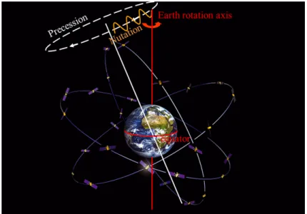
2.2.7 Nutation and Precession . . . 17
2.2.8 Azimuth and Elevation . . . 18
2.3 Clean Space . . . 20
2.4 5G- Satellites . . . 22
3 Orbit Dynamics 25 3.1 The Kepler’s Laws . . . 25
3.2 The Newton’s Laws . . . 29
3.2.1 Newton’s Universal Law of Gravitation . . . 29
3.3 Simulation Results . . . 30
4 Spacecraft Kinematics and Dynamics 33 4.1 Attitude kinematics of a spacecraft . . . 33
4.1.1 Euler Angle Kinematics . . . 33
4.1.2 Quaternion Kinematics . . . 34 4.2 Attitude Dynamics . . . 35 4.3 Internal Torques . . . 36 4.3.1 Reaction Wheels . . . 37 4.3.2 Thruster . . . 38 4.4 External Torques . . . 38 4.4.1 Magnetic Torque . . . 38
5 Filtering for Attitude Estimation and Calibration 41
5.1 Background . . . 41
5.1.1 Static-Based and Filter-Based Estimation . . . 41
5.1.2 State Estimation Techniques . . . 42
5.2 Attitude Representation for Kalman filtering . . . 44
5.2.1 Three-Component Representation . . . 44
5.2.2 Adaptive Quaternion Representation . . . 44
5.2.3 Multiplicative Quaternion Representations . . . 45
5.3 Attitude Estimation . . . 45
5.3.1 Extended Kalman Filter . . . 45
5.3.2 Murrell’s version . . . 47 5.4 Simulation Results . . . 49 6 Attitude Control 53 6.1 Control background . . . 53 6.1.1 State Models . . . 53 6.1.2 Control Theory . . . 54
6.2 Single Axis Attitude Control . . . 55
6.2.1 Stability of Nonlinear Dynamic Systems . . . 55
6.3 Attitude Control: Reaction Wheels . . . 56
6.3.1 Lyapunov’s Direct Method . . . 57
6.4 Simulation Results . . . 58
7 Space Rendezvous 69 7.1 Space Rendezvous Background . . . 69
7.2 Relative Dynamics . . . 70
7.3 Rendezvous Trajectory . . . 71
7.4 Simulation Results . . . 72
8 Conclusions and Future Work 77 8.1 Conclusions . . . 77
8.2 Future Work . . . 78
List of Figures
1.1 Sun-synchronous orbit. . . 1
1.2 Spacecraft system. . . 2
2.1 Copernicus programme . . . 5
2.2 Land monitoring service . . . 6
2.3 Marine monitoring service . . . 6
2.4 Land monitoring service . . . 7
2.5 Climate monitoring service . . . 7
2.6 Emergency . . . 8
2.7 Sentinel-6 . . . 8
2.8 Sentinel-6 . . . 9
2.9 Sun-synchronous orbit. . . 10
2.10 Example of Earth-centered Inertial frame. . . 11
2.11 Example of Earth-centered Earth-fixed frame. . . 11
2.12 Example of Orbit frame. . . 12
2.13 Example of Orbit frame. . . 12
2.14 Coordinate frames related. . . 13
2.15 Example of injection trajectory. . . 14
2.16 Example of a CESS. . . 15
2.17 How the CESS works. . . 15
2.18 Example of star tracker. . . 16
2.19 example of an image captured by STR. . . 16
2.20 The difference between Nutation and Precession. . . 18
2.21 Elevation and azimuth. . . 19
2.22 Satellites into Earth’s orbit. . . 20
2.23 e.Deorbit mission. . . 21
2.24 5G-satellite . . . 22
2.25 Network ecosystem . . . 23
3.1 First Kepler Law . . . 25
3.2 Kepler elements . . . 26
3.3 Second Kepler Law . . . 28
3.4 Satellite with a sun-synchronous orbit. . . 30
3.5 Sun-synchrnous satellite around the Earth. . . 31
3.6 Satellite position. . . 32
3.7 Satellite distance relative to the center of the Earth with the Newton Laws. . . 32
5.1 Proper Euler Angles . . . 44
5.3 Estimator Extended Kalman Filter Quaternions Errors. . . 49
5.4 Estimator Extended Kalman Filter Quaternions Errors. . . 50
5.5 Estimator Extended Kalman Filter Quaternions Errors. . . 51
6.1 Negative feedback control block diagram. . . 54
6.2 Controller quaternions. . . 59
6.3 Angular velocity of reaction wheels. . . 60
6.4 Torque of reaction wheels. . . 61
6.5 Nonlinear control law. . . 62
6.6 Controller quaternions erros with kp=10. . . 63
6.7 Controller quaternions erros with kp=30. . . 64
6.8 Controller quaternions erros with kp=200. . . 65
6.9 Controller quaternions erros with kd=50. . . 66
6.10 Controller quaternions erros with kd=200. . . 67
6.11 Controller quaternions erros with kd=800. . . 68
7.1 Spacecraft rendezvous process. . . 69
7.2 Example of burns to trajectory rendezvous. . . 71
7.3 Mission sequence of the simulation. . . 72
7.4 Results of space rendezvous. . . 73
7.5 Final position and velocity of both spacecrafts. . . 74
7.6 Evolution of the x coordinate position of spacecraft in red and the target spacecraft in green. . . 74
7.7 Evolution of the y coordinate position of spacecraft in green and the target space-craft in red. . . 74
7.8 Evolution of the z coordinate position of spacecraft in red and the target spacecraft in blue. . . 75
List of Tables
5.1 Continuous-discrete linear Kalman filter. . . 43 5.2 Extended Kalman Filter for attitude estimation. . . 47
Glossary
ADCS Attitude determination and control subsystem
CESS Coarse Earth and Sun Sensors
C-W Clohessy-Wiltshire
PD control Proportional-Derivative controller RODC Rendezvous orbital dynamics and control SISO Single-input-single-output
SSO Sun-synchronous orbit
STR Star Tracker
ODE Ordinary differential equation ORION On-orbit servicing and navigation OSS On-orbit servicing of satellites
Chapter 1
Introduction
1.1 Context
We depend directly or indirectly on satellites to communicate, entertainment, information and so much more.
Since the beginning of the space exploration, satellites have been good tools to study solar sys-tem and other syssys-tems. Syssys-tems interact with the environment and with other syssys-tems. Sometimes, we can ignore those interactions between systems when testing software and integrated electronic equipment. However, when we deal with control systems, open loop testing is inadequate be-cause only hardly could one effectively and efficiently define an adequate combination of inputs and expected outputs. Therefore, some systems require closed loop testing and that implies to sim-ulate external systems, the system under test interacts with the environment and systems dynamics. The satellite’s sun-synchronous orbits travels from north to the south poles while the Earth turns and the satellite pass at the same time every day through the same region of the Earth (see Figure 1.1). Those orbits are very useful for weather satellites, climate studies, imaging and to control human activity.
Figure 1.1: Sun-synchronous orbit. Source: [55]
Unfortunately, the satellites have a limited life time and when they are inoperative many con-tinue to orbit around the Earth. When obsolete satellites do not decay, they are consequently just getting in the way of another satellite. Over the years debris has accumulated around the Earth. Now, ESA has been studying new measures to remove the debris and promote green technologies.
1.2 Goals
The main goal of this Dissertation is to analyse and to implement a Sun-synchronous satellite system, see figure 1.2.
Figure 1.2: Spacecraft system. Particular points that will be addressed in simulation include:
• implementation and simulation of the spacecraft relative positions of the Earth with New-ton’s Laws;
• implementation the actuators of a spacecraft;
• implementation kinematics and dynamics of a spacecraft; • implementation and simulation of the attitude estimation;
1.3 Motivation 3
1.3 Motivation
Satellites are more important to our lives than we may think. With the study of satellites we can improve our life quality. For example, without satellites we could not have wireless communica-tions like cellphones nor smartphones with internet connection nor we could watch live TV from the other side of the Earth.
Nowadays many people in the morning use their mobile phone to get updated on the news and to check those little things are already part of our routine that we do without even realise how much technology we need just to know the weather. For these reasons and many other, it is very important to study satellites and their orbits.
However, there are many satellites that are obsolete and now they are just debris. To continue the space exploration we need to implement new measures and adopt to green technologies. We also need to apply this measures if we want to continue to live as we are living nowadays.
1.4 Organization of the Dissertation
This Dissertation is divided into eight chapters. The first chapter is a contextualisation of Dis-sertation, objectives and motivation. We then provide an introduction to Copernicus programme and bibliographical review of some concepts. In the third chapter we present a brief survey of orbit dynamics and the difference between the Kepler’s Laws and Newton’s Universal Law of Gravitation. The fourth chapter is dedicated to the kinematics and dynamics of a spacecraft. Also in fourth chapter we present the actuators implementation in a spacecraft. The fifth chapter is dedicated to the attitude estimation of a spacecraft using the filter estimation. Then, in the next chapter we present the attitude control of a spacecraft. The seventh chapter is dedicated to the space rendezvous. Finally, the eighth chapter describes the main conclusions and future work.
Chapter 2
Literature Review
This chapter begins with a brief introduction of Copernicus programme, theory of sun-synchronous orbit, clean space and 5G-satellites.
2.1 Copernicus programme
This dissertation is inspired by the Copernicus program. Whose main goal is to observe the en-vironment, collect and analyze data and provide equipment to improve the state of planet Earth. There is a set of Sentinel satellites that are part of this program. Each Sentinel satellite has a specific role in monitoring changes in soil, oceans and atmosphere. So far Sentinel-1, Sentinel-2, Sentinel-3 Sentinel-4, Sentinel-5 are in orbit. And Sentinel-6 and EarthCARE are still in construc-tion phase.
Figure 2.1: Copernicus programme Source: [56]
As shown below each Sentinel and EarthCARE satellites mission has a specific mission:
• Sentinel-1: land monitoring changes by collecting data on geographic information;
Figure 2.2: Land monitoring service Source: [57]
• Sentinel-2: Marine monitoring changes;
Figure 2.3: Marine monitoring service Source:[58]
2.1 Copernicus programme 7 • Sentinel-3: Atmosphere monitoring changes;
Figure 2.4: Land monitoring service Source: [59]
• Sentinel-4: Climate monitoring changes;
Figure 2.5: Climate monitoring service Source: [60]
• Sentinel-5: Emergency management service;
Figure 2.6: Emergency Source: [61] • Sentinel-6: security service;
Figure 2.7: Sentinel-6 Source: [62]
2.1 Copernicus programme 9 • EarthCARE: Earth Cloud Aerosol and Radiation Explorer satellite mission;
Figure 2.8: Sentinel-6 Source: [63]
2.2 Sun-Synchronous Orbit
Sun-synchronous orbit allow the satellite pass in the same area of the Earth at the same solar time and ranges from 200 to 1680 km altitude wise and passes near the poles[50]. This type of orbit in relation to the sun is fixed. Whereas that Earth does a complete turn around the sun (360o) per
year, the spacecraft move 1oper day to compensate. Sun-synchronous orbit is useful for mapping,
weather satellites and communication satellites.
For the spacecraft to have an sun-synchronous orbit it needs to maintain a height and the re-spective orbital inclination. If one of this parameters changes the spacecraft no longer have a sun-synchronous orbit.
Figure 2.9: Sun-synchronous orbit. Source: [64]
2.2.1 Coordinate Frames
To represent the different types of objects, for example Moon, Earth and satellite, we have a diver-sity of coordinates frames.
2.2 Sun-Synchronous Orbit 11 • Earth-centered Inertial (ECI)- Their origin is at the center of Earth.
Figure 2.10: Example of Earth-centered Inertial frame. Source: [65]
• Earth-centered Earth-fixed (ECEF)- Like ECI, their origin is at the center of Earth, but now the x-axis and y-axis rotate with same angular velocity as Earth. In other words, the coordinates at a given fixed point does not change with the rotation of the Earth.
Figure 2.11: Example of Earth-centered Earth-fixed frame. Source: [66]
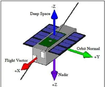
• Orbit Satellite frame- Their origin is at the center of satellite, where the x-axis represents the direction of the velocity of the satellite, z-axis point to the center of the Earth and the y-axis completes the set of coordinates axis.
Figure 2.12: Example of Orbit frame. Source: [67]
• Satellite Body frame- Their origin is at the center of satellite and it is useful to represent the satellite in space.
Figure 2.13: Example of Orbit frame. Source:[68]
2.2 Sun-Synchronous Orbit 13
2.2.2 Coordinate Transformations
A coordinate transformation is a mapping that relates the representation in one coordinate system to another. For example, transforming a Cartesian coordinate system into another coordinate sys-tem is done by rotating on each of the coordinate axes. In that case, the three rotational matrices are: Px(a) = 2 6 4 1 0 0 0 cosa sina 0 sina cosa 3 7 5 (2.1) Py(a) = 2 6 4 cosa 0 sina 0 1 0 sina 0 cosa 3 7 5 (2.2) Pz(a) = 2 6 4 cosa sina 0 sina cosa 0 0 0 1 3 7 5 (2.3)
wherea corresponds to the counter-clockwise angle on each axis.
Figure 2.14: Coordinate frames related. Source: [31]
2.2.3 Injection Trajectory and angular velocity
To be in orbit, the spacecraft needs to have an injection trajectory and an angular velocity. To determine the relative position of Earth, Moon and Sun we need to know a calendar date,
With the specified calendar date we can know the altitude and inclination of spacecraft. It is necessary to have an angular velocity to maintain the height and control spacecraft orbit’s.
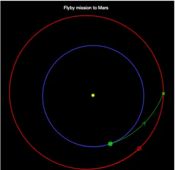
The injection trajectory is the trajectory that spacecraft will make until it arrive to the planet or near-Earth object (NEOs). For example, if we want the spacecraft to arrive to Mars the injection trajectory will trace the route that the spacecraft will make.
Figure 2.15: Example of injection trajectory. Source: [69]
2.2.4 CESS
The Coarse Earth Sun Sensor (CESS) provides an omnidirectional coarse estimation of Earth and Sun position in the satellite reference frame [44].
CESS have two sensors, thermistors, which heat in different ways when they are exposed to solar or infrared emissions emitted by Sun and reflected by Earth, Earth Albedo. The output of CESS is given in Ohms.
The Earth Albedo is the reflecting power of a surface and it has a scale from zero to one. The lower albedo is, the more sun radiation is absorbed. As well as, the bigger albedo is, the less sun radiation is absorbed. The albedo allows scientists to study climate change and the changes in the Earth’s surface [70].
2.2 Sun-Synchronous Orbit 15 Furthermore, from the study of albedo, we can know some properties of planets or asteroids. For example, one can find out the type of surface and this way, if there is ice outside the Earth.
Figure 2.16: Example of a CESS.
Source: http://www.spacetech-i.com/products/satellite-equipment/cess-a-cess
To determine the relative position of Earth and Sun vector, the CESS uses six orthogonal axis, while measures the temperatures and estimate the irradiated infrared emissions and solar flux.
Figure 2.17: How the CESS works.
Source: http://www.spacetech-i.com/products/satellite-equipment/cess-a-cess
2.2.5 Star Tracker
The Star Tracker or simply STR is an optical attitude measurement devices [48] as CESS, how-ever, the STR has more accuracy. Since ancient times, the humans used reference stars to help navigate. Nowadays, this is very useful to spacecraft navigation. Furthermore, there is a list of
Figure 2.18: Example of star tracker. Source: [72]
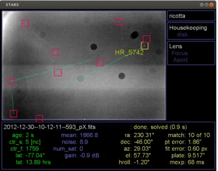
From an image captured from the stars, the STR can estimate the position in the reference frame of the spacecraft because of differences between the captured imaged with the stars and their absolute position from a star catalog [73].
To compute the altitude, inclination or angular velocity we need to observe the changes of star’s positions relative to the satellite over time.
Figure 2.19: example of an image captured by STR. Source: [73]
2.2 Sun-Synchronous Orbit 17
2.2.6 Earth Magnetic Field
Spacecraft in Earth orbit use magnetometers as attitude control sensors. The magnetometer is an sensor that measures the flux of the magnetic field.
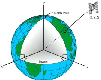
To calculate the magnetic field in Cartesian coordinates, we need to know the spacecraft’s co-ordinates in space (x, y, z). Also, we need to calculate the distance from spacecraft to the center of the Earth.
r = x2+y2+z2 12 (2.4)
Also, we need to know radius of Earth (R) and the constant M, that it is equal to 31000 nT R3.
Bx=3xzM r5 ;By= 3yzM r5 ;Bz= 3z2 r2 M r5 (2.5)
2.2.7 Nutation and Precession
Nutation and Precession are the motion of the Earth’s axis and they are periodic [1].
The Nutation is the angle that the axis Earth’s axis makes with the reference frame [1]. This mo-tion is due to the gravitamo-tional attracmo-tion of Sun and Moon.
The Precession is a change in the orientation of the rotational axis of the Earth. In other words, Precession is the changes Earths rotational axis. Like Nutation the cause of the Precession is
grav-Figure 2.20: The difference between Nutation and Precession. Source: [74]
2.2.8 Azimuth and Elevation
Over time the spacecraft in orbit needs to communicate with the ground stations to send or receive data. As ground stations are fixed to the ground it is essential to know the visibility windows be-tween spacecraft and ground stations. The main telecommunications device of the ground stations is the parabolic antenna.
To calculate the visibility windowns between spacecraft and ground stations we need to know: azimuth, elevation and great-circle distance.
• The azimuth is the horizontal angular distance between the North and a star, measured in degrees [75].
cosa = sinhcosb
sing (2.6)
In this case, we assume that the Earth is a sphere, a is the azimuth angle, the b is actual spacecraft declination, theg is the zenith angle (is one point over the ground stations) and lastly, h is the hour angle.
2.2 Sun-Synchronous Orbit 19 • The elevation or altitude is the vertical angular distance between a star and the ground.
Figure 2.21: Elevation and azimuth. Source: [76]
• Great-circle distance is the minimum distance between two points on the surface of the Earth. With great-circle distance we can calculate the visibility windowns between space-craft and ground stations.
a = sin2✓Df 2
◆
+cosf1⇥ cosf2⇤ sin2✓Dl
2 ◆
(2.7) Thef is the latitude, l is the longitude from one point, and Df and Dl are the difference, respectively, of the latitude and longitude between two points.
c = 2 ⇥ tan2⇣pa,p(1 a)⌘ (2.8)
2.3 Clean Space
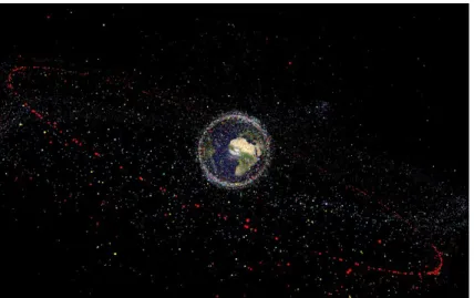
As previously described, satellites are essential to our daily life and over the years the number of satellites is accumulating on Earth’s orbit. Presently there are more than 6000 satellites in orbit. Between then, only less than an hundred are fully operational, that number corresponds 6% of all the satellites around the Earth. With time the satellites that are obsolete could explode and their fragments or mission-related objects are a problem for the next space missions. Therefore colli-sions between functional and obsolete satellites are a reality and this can cause even more space debris, can lead some missions to failure and that is very expensive. The space debris is a major risk for space missions [40] .
Figure 2.22: Satellites into Earth’s orbit. Source: [77]
ESA recently has an initiative to clean space so that space exploration could continue and there is no space debris. Thus, the three solutions proposed by Esa [78] are:
• EcoDesign: promote green technologies and and study environmental impacts; • CleanSat:reduce production of space debris;
• eDeorbit: remove space debris from orbit;
e.Deorbit will be launched by 2023 and its main mission will be de-orbit debris with an alti-tude of less than 600 km, re-orbit debris with a altialti-tude of more than 2000km and finally, allow the controlled re-entry of debris into the Earth’s atmosphere that within 25 years debris does not decay.
2.3 Clean Space 21
Figure 2.23: e.Deorbit mission. Source: [79]
The target must not have a mass exceeding eight tonnes, it has to be obsolete and with sun-synchronous orbit. As the mission of e.Deorbit is to remove several targets, it must be able to evaluate several types of targets at a distance. For that it will need:
• navigational systems; • cameras;
• propulsion system; 1. chemical; 2. electrical;
• capture technique (could be): 1. robotic arm;
2. tentacles; 3. net;
4. ion-beam shepherd;
In this Dissertation we will study the e.Deorbit solution, in particular the guidance navigation and control of e.Deorbit from phase that knows what the target is until its capture.
The target orbit is determined by RADAR sensors that are on the ground and when the e.Deorbit is relatively close to the target, the distance between the two is obtained through the relative navi-gation stars, [29].
2.4 5G- Satellites
The 5th generation wireless systems, also called 5G, is the next communications system. The 5G will have an higher bandwidth capacity, more secure communications and allows a greater number of users to have a data rate of 10Gb/s. Also, the 5G intends to have a latency lower than 4G and save the battery consumption.
The 5G-Satellites will play a very important role in the implementation of 5G. For example, security, transport service, coverage and public safety. With 5G-satellites it is possible to provide communications in the most isolated areas but also guarantee communications in areas requiring additional capacity [39].
Figure 2.24: 5G-satellite Source: [80]
The networks will have an higher speed due to use of millimeter wave band transmission. No-tice that, data is transmited over radio waves and one of properties of electromagnetic waves is that the higher the frequency is, the smaller its wavelength is. Also, the higher the frequency the more data it can transmit. Therefore, the millimeter wave uses a band between the 30 GHz and 300 GHz so the wavelength is in the range of milimeters [24].
As previously stressed, satellites will play a very important role in the implementation of 5G technology, and in particular for:
• Coverage and integration; • resilience;
• content multicast and caching;
• internet of things over satellite network; • higher user mobility;
2.4 5G- Satellites 23
Figure 2.25: Network ecosystem Source:[30]
With satellites it is possible to provide greater network coverage. If some terrestrial cells are at their maximum capacity through a network configuration software satellites can provide network to the cells [30].
Chapter 3
Orbit Dynamics
This chapter provides a brief survey of orbit dynamics. We start with the Kepler’s laws, that pro-vides a description of the motions of the planets in the solar system, but they do not explain why the planets move in that way. Next, we present the Newton’s Universal Law of Gravitation that combined with the Newton’s Laws of Motion can be used to explain the original Kepler’s law.
3.1 The Kepler’s Laws
Johannes Kepler began as Tycho Brahe’s helper and student. During most of his life, Tycho Brahe recorded the positions of the planets over time. This recorded data turned out to be instrumental for the findings of Kepler. Indeed, when Kepler was analyzing the data, he found interesting rela-tions, that are current summarized as the three laws of Kepler:
• First Law: The orbit of the planets around the sun is elliptical.
Figure 3.1: First Kepler Law Source: [81]
See Fig. 3.1, where in this case the sun is the primary. The body that is centered with the reference point used is called as primary, while the other body is designated as secondary. The Kepler elements that characterize the trajectories (see Fig. 3.2) are used in non-inertial trajectories and centered on one of the bodies.
Keplerian elements:
– e - eccentricity of orbit;
Ife is equal to zero the orbit is a circle, or if e is between zero and one the orbit is an ellipse and for the last case, ife is bigger than one the orbit is a parable.
– a - semi-major axis of the planet’s orbit; – P - perihelion;
– i - angle between plane of the Sun’s equator and planet’s orbit; – w - longitude of perihelion;
– W - longitude of ascending node;
Figure 3.2: Kepler elements Source: [11]
From the Kepler elements one can compute the distance from the planet to the sun. To this effect, we need to perform the following calculations.
3.1 The Kepler’s Laws 27 First, we need to calculate the eccentric anomaly. Considering that the equation of an ellipse is given by, x2 a2+ y2 b2 =1 (3.1) It follows that, cos(E) = x a (3.2) and sin(E) = y b, (3.3)
where E is the eccentric anomaly, a is the semi-major axis and b is the semi-minor axis.
From this, the mean anomaly (denoted by M) and the angle of planet from perihelion (de-noted byn) are obtained as:
M = E esin(E) (3.4) n = 2tan 1 r 1 +e 1 etan ✓E 2 ◆! (3.5)
Lastly, the calculation of the distance between the planet and the Sun, denoted by r, is given by
r = a 1 e2
1 +ecosn, (3.6)
• Second Law: A line segment joining a planet and the Sun sweeps out equal areas during equal intervals of time, see Fig. 3.3. This means that the orbit velocity of the planet is not
Figure 3.3: Second Kepler Law Source: [82]
• Third Law: The square of the orbital period T of a planet is proportional to the the cube of the semi-major axis of the orbit of the planet, that is,
T2µ a3 (3.7)
Satellite’s Position
To find the position of a satellite with the Kepler’s Laws using the Heliocentric Ecliptic coordinates (x, y, z) one get,
x = r(cos(W)cos(w + n) sin(W)sin(w + n)cos(i)) (3.8)
y = r(sin(W)cos(w + n) + cos(W)sin(w + n)cos(i)) (3.9)
z = r sin(W)sin(w + n)cos(i) (3.10)
To obtain in the Heliocentric Equatorial coordinates(X,Y,Z), we need to perform the following
transformation 2 6 4 X Y Z 3 7 5 = 2 6 4 1 0 0 0 cos(i) sin(i) 0 sin(i) cos(i) 3 7 5 2 6 4 x y z 3 7 5 (3.11)
Although Kepler’s laws were an advance for the study of the satellite’s orbit, these laws are based on data that Tycho Brahe registered to that of time [83] and as such do not explain why the
3.2 The Newton’s Laws 29 orbits of the planets move in this way.
3.2 The Newton’s Laws
Years later, in 1687, Isaac Newton presented his Universal Law of Gravitation through Kepler’s Third Law.
3.2.1 Newton’s Universal Law of Gravitation
The Newton’s universal equation of gravity says basically that the force F of attraction between two bodies of mass M and m is proportional to the product of the two masses, and inverse propor-tional to the square of the distance r between them. For the example case of Earth with mass M and Moon with mass m, one has
F = GmM
r2 , (3.12)
where, G is the gravitational constant the value 6.670⇥10 11.and r is the distance between Moon
and the Earth.
Third Law of Kepler from Newton’s Universal Law of Gravitation
Kepler’s third Law can be derived from applying the Laws of Motion and Newton’s universal equation of gravity. We can see more in detail at [2].
For simplify the calculation it consider that the rigid body has a circular orbit around the Earth. Applying the Laws of Motion on the rigid body in circular motion this force is denoted by cen-tripetal force:
Fc=mv 2
R, (3.13)
where, the mass of the rigid body is denoted by m, the orbital velocity is denoted by v and distance R in the circular motion is the semi-major axis a.
As the motion of the rigid body is circular, the velocity can be described by the space traveled to divided by the time that the rigid body takes to take a turn. Following, the space traveled can be defined by 2p R, where R is the distance from rigid body to the Earth.
If we equate the gravitational force with the centripetal force one get,
GMm
R2 =
mv2
R (3.15)
If we resolve the last equation in function of period, T , is given by,
T2= 4p
2
G(M + m)R3, (3.16)
where, T is the period of the rigid body (in Earth years).
3.3 Simulation Results
In this Section we illustrate through computer simulations the evolution of the satellite’s position relative to the Earth.
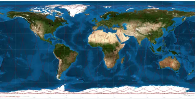
Through the tool developed by NASA called by General Mission Analysis Tool, GMAT, it was simulated the satellite sun-synchronous orbit around the Earth over a period of one day.
The results obtained for the satellite’s position (see figures 3.4 and 3.5) has as reference point the center of the Earth.
3.3 Simulation Results 31
Figure 3.5: Sun-synchrnous satellite around the Earth.
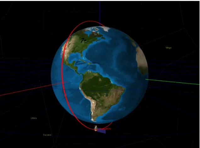
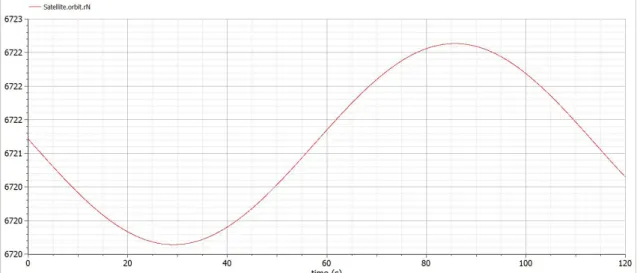
The following figures show the positions of the satellite relative to the center of the Earth. In the figure 3.7, the result obtained was through the OpenModelica tool.
The distance of the satellite from the center of the Earth (denoted by r) throught Newton’s laws is given by,
r =
L2
GMm2
1 + ecosq (3.17)
where, L is the angular momentum of the satellite, mass of the Earth is denoted by M and the mass of satellite is denoted by m. It possible see the deduction of the equation (3.17) in [4]. Also, note that the angular momentum of a satellite is calculate by the equation (4.14).
Figure 3.6: Satellite position.
The following are the results of the distance of the satellite from the center of the Earth through Newton’s laws.
Figure 3.7: Satellite distance relative to the center of the Earth with the Newton Laws. See figure 3.7, the distance changes along the time because Newton’s Laws takes into account the forces applied to the satellite. Contrary, the Kepler’s Laws are based on collected data and the distance is constant along the time.
Chapter 4
Spacecraft Kinematics and Dynamics
This chapter is dedicated to the kinematics and dynamics of a spacecraft.
In Section 4.1 we present the attitude kinematics of a spacecraft. The attitude kinematics is rep-resented first by Euler angles and after by quaternion. Section 4.2 is dedicated to the spacecraft’s dynamic. To calculate attitude dynamic of spacecraft it is used angular momentum, rigid body dymamics and motion and Euler’s equation of motion. In Section 4.3 we present the actuators that create the internal torques of the spacecraft, and finally in Section 4.4 we present the actuators that create the external torque of the spacecraft.
4.1 Attitude kinematics of a spacecraft
This Section introduces the two main representation of the attitude of a spacecraft: Euler Angle Kinematics and Quaternion Kinematics.
4.1.1 Euler Angle Kinematics
Euler angle is used to represent a rotation of the spacecraft. Representing the attitude kinematics by the Euler angle is easier to develop and to visualise but it uses a lot of computational power. And it is not successful method to describe attitude dynamics of a spacecraft. We can see the deduction of the Euler angle kinematics in [12].
2 6 4 ˙ q1 ˙ q2 ˙ q3 3 7 5 =cos1q 2 2 6 4
cosq2 sinq1sinq2 cosq1sinq2
0 cosq1cosq2 sinq1cosq2
0 sinq1 cosq1 3 7 5 2 6 4 w1 w2 w3 3 7 5 (4.1)
4.1.2 Quaternion Kinematics
Quaternion representation have four components vector. The quaternion (denoted by q) has two parts, the first part consists of three-vector part and a scalar part, that is,
q = " q1:3 q4 # (4.2) where q1:3= 2 6 4 q1 q2 q3 3 7 5 (4.3)
The representation of the quaternions is based on the Euler rotational theorem. Representing the attitude kinematics by quaternions there are several advantages for example, to the successive rotations can be resolved by quaternions multiplicative [13] and [10]. To determine the attitude of spacecraft it is necessary to integrate the quaternions kinematic equation
2 6 6 6 6 4 ˙q1 ˙q2 ˙q3 ˙q4 3 7 7 7 7 5= 1 2 2 6 6 6 6 4 0 w3 w2 w1 w3 0 w1 w2 w2 w1 0 w3 w1 w2 w3 0 3 7 7 7 7 5 2 6 6 6 6 4 q1 q2 q3 q4 3 7 7 7 7 5 (4.4)
where, the angular velocity, denoted byw, evolves according to the by dynamics equations. The compact form to represent the quaternion kinematics of the satellite is
˙q =1 2W(w)q (4.5) so that, W(w) = " [w⇥] w wT 0 # (4.6)
4.2 Attitude Dynamics 35
4.2 Attitude Dynamics
Angular MomentumIn order to obtain the angular acceleration we need to compute the angular momentum.
To calculate the angular momentum (denoted by H) of the spacecraft, first it is necessary to compute the momentum of inertia matrix (denoted by I). The momentum of inertia matrix is the inertia (difficulty of motion) of the body has to rotation around the axis.
The moment of inertia matrix is given by
I = 2 6 4 Ixx Ixy Ixz Iyx Iyy Iyz Izx Izy Izz 3 7 5 (4.7)
where the components of moment of inertia matrix are given by, Ixy=Iyx= Z Z Z xydm (4.8) Ixz=Izx= Z Z Z xzdm (4.9) Iyz=Izy= Z Z Z yzdm (4.10) Ixx= Z Z Z (y2+z2)dm (4.11) Ixz= Z Z Z (x2+z2)dm (4.12) Ixz= Z Z Z (y2+x2)dm (4.13)
From the moment of inertia, I, and the angular velocity of the satellite denoted byw, we obtain the angular momentum as
2 6 4 Hx Hy H 3 7 5 = 2 6 4 Ixx Ixy Ixz Iyx Iyy Iyz I I I 3 7 5 2 6 4 wx wy w 3 7 5 (4.14)
Euler’s equation of motion
Using a body fixed reference to the satellite, we can now apply the Euler’s equation of motion [9], 2 6 4 L M N 3 7 5 = d~Hdt |B+ ~w ⇥ ~H (4.15) = 2 6 4 Ixx Ixy Ixz Iyx Iyy Iyz Izx Izy Izz 3 7 5 ⇥ 2 6 4 ˙ wx ˙ wy ˙ wz 3 7 5 + 2 6 4 Ixx Ixy Ixz Iyx Iyy Iyz Izx Izy Izz 3 7 5 ⇤ 2 6 4 wx wy wz 3 7 5 (4.16) = 2 6 4 +Ixxw˙x Ixyw˙y Ixzw˙z Iyxw˙x+Iyyw˙y Iyzw˙z Izxw˙x Izyw˙y+Izzw˙z 3 7 5 + ~w ⇥ 2 6 4 +wxIxx wyIxy wzIxz wxIyx+wyIyy wzIyz wxIzx wyIzy+wzIzz 3 7 5 (4.17) = 2 6 4 Ixxw˙x Ixyw˙y Ixzw˙z+wy(wzIzz wxIxz wyIyz) wz(wyIyy wxIxy wzIzz) Iyyw˙y Ixyw˙x Iyzw˙z wx(wzIzz wyIyz wxIxz) +wz(wxIxx wyIxy wzIxz) Izzw˙z Ixzw˙x+Iyzw˙y+wx(wyIyy wxIxy wzIyz) wy(wxIxx wyIxy wzIxz) 3 7 5 (4.18)
where, ˙w is the angular acceleration of the satellite in the body frame.
To simplify the calculation, we consider that the moment of inertia of the spacecraft has two planes of symmetry [8], which implies
Iyz=Ixy=Ixz=0 (4.19)
The forme simplify of Euler’s equation is given by, 2 6 4 L M N 3 7 5 = 2 6 4 Ixxw˙x+wywz(Izz Iyy) Iyyw˙y+wxwz(Ixx Izz) Izzw˙z+wxwy(Iyy Ixx) 3 7 5 (4.20)
4.3 Internal Torques
Internal torques are created by the spacecraft actuators causing a change in angular momentum. In this dissertation we consider for the actuators the reaction wheels and thrusters that create internal torques. Reaction wheels are commonly used for attitude control while the thrusters are used to orbit control.
4.3 Internal Torques 37
4.3.1 Reaction Wheels
In order to determine the total angular momentum of the spacecraft with the reaction wheels we need to calculate the moment of inertia of the spacecraft with and without the wheels. The wheels are distinguish by l and considering that are n reaction wheels in the spacecraft.
Each reaction wheel rotates around the spin axis, thus the wheel is axially symmetric about its spin axis [12].
The equation for the calculation of the moment of inertia of wheel (denoted by Jw
l ) is given by
Jlw=Jl?(I3 wlwTl ) +JlkwlwTl , (4.21)
where wl is the unit vector that defines the spin axis relative to the body frame, I3 is the 3 ⇥ 3
identity matrix, J?
l and Jlkare the moment of inertia perpendicular and parallel, respectively, to the
spin axis.
To calculate the total moment of inertia with and without wheels we need to sum all the mo-ment of inertia of the wheels and the momo-ment of inertia of spacecraft without wheels, one get
J = ˜J +
Â
nl=1
J?
l (I3 wlwTl ) (4.22)
and the angular momentum of the wheel, denoted by Hw, along the spin axes is given by,
Hw=
Â
n l=1 Jk l(wlw + wlw)wl⌘ nÂ
l=1 Hw l wl (4.23)Therefore, the total angular momentum, denoted by H, of the spacecraft is H = ˜Jw +
Â
nl=1
Jlw(w + wlwwl) =Jw + Hw (4.24)
where,ww
l is the angular velocity of the wheel,w is the angular velocity of the spacecraft, ˜Jis the
moment of inertia without wheels and J is the moment of inertia of the wheels just in the trans-verse spin axes and not along spin axes.
The first part of the equation, see equation (4.22), corresponds to moment of inertia of the spacecraft without the wheels and the second part is the moment of inertia of wheels.
˙ Hw= n
Â
l=1 ˙ Hlwwl = nÂ
l=1 Lwl wl⌘ Lw (4.25)The rotation kinetic energy, denoted by Ecof a spacecraft with the reaction wheels is given by,
Ec=1 2(w)TJw + 1 2 n
Â
l=1 (Jlk) 1(Hlw)2 (4.26) 4.3.2 ThrusterThe thrusters are used to attitude control and orbit control, thus the torques (denoted by L) and forces (denoted by F) are applied on the spacecraft.
F = ˙mvrel, (4.27)
and
L = r ⇥ F (4.28)
where ˙m is the fuel mass loss rate, vrel is the velocity of the removed mass relative to the
space-craft, r is the vector distance of the thruster to the spacecraft center of mass.
See in equation (4.27), the reaction force is on the spacecraft, so with the third law of motion the sign is negative.
4.4 External Torques
External torques are created by different mechanisms external to the spacecraft. In this dissertation we only consider magnetic dipole that create external torques.
4.4.1 Magnetic Torque
In order to calculate the torque (denoted by L) one need to compute the magnetic dipole (denoted by m), which is given by
m = NIA, (4.29)
where, the number of wire loops is denoted by N, I is the current in amperes[A] and A is the area of the wire loop.
4.4 External Torques 39 Now it is possible to determine the torque generated by magnetic dipole in body frame,
L = m ⇥ B (4.30)
Note that the magnetic torques can only control two axis each time. In other hand, the mag-netic torques do not create forces thus they do not change the orbit of the spacecraft.
Chapter 5
Filtering for Attitude Estimation and
Calibration
This chapter is dedicated to the attitude estimation of a spacecraft using the filter estimation. Section 5.1 provides a review of estimation theory, the differences between static-based and filter-based estimation. Also, it reviews some filter estimations, for instance the Kalman filter for linear systems and the extended Kalman filter for nonlinear systems. We will focus on the filter estima-tion because the model of the system is a dynamic model. Secestima-tion 5.2 presentes three different representations of spacecraft attitude: three-component representations, additive quaternion rep-resentation and multiplicative quaternion reprep-resentations as well as the advantages and disadvan-tages for different possibilities for the representations. In Section 5.3 we will see the description of the implementation and the differences between the Extended Kalman Filter and the Murrell’s version. Lastly, Section 5.4 presents the simulation results for the attitude estimation of a space-craft.
5.1 Background
This Section provides a brief review of estimation theory in the context of this dissertation as well, the differences between the estimations methods for linear and nonlinear systems. All methods of the estimation requires the sensor measurements to estimate unknown variables.
5.1.1 Static-Based and Filter-Based Estimation
The filter-based estimation to determine the current state of a system needs the previous time state and the sensors measurements, for example, the magnetometers sensors. The measurements are usually has corrupted by noise, which will be assumed to be Gaussian random noise.
The filter estimation could be applied to filter noisy measurement observations and the estima-tion quantities [12].
The static estimation can be used for initial estimate on the filter estimation or to verify the results of the filter estimation.
The advantages of using the static-based estimation are the fact that usually require less com-putationally effort and the estimation is better approximated to the desired solution. The main disadvantage is the need to have for each time the full observability so that the solution can be computed without algebraic singularities [13].
The advantages of using filter-based estimation techniques are the fact that a solution can be determined when exist algebraic singularity situations. Because one can include another state es-timation variables from the nearby past. In case of attitude determination of a spacecraft, biases are included into the state estimation. Also for the previous case, the estimate error covariances is added to the solution. The disadvantage is that to determine a solution it is necessary the previous state. Also, in the comparison with the static estimation the filter estimation is computationally slower [12].
The definition of the covariance matrix is each element of the matrix in the ith row and jth
column is the covariance between the ith and jthvariables. The diagonal elements of the matrix
are the variance of this variable. The covariance between this two variables is a measure of the joint variability of two random variables.
5.1.2 State Estimation Techniques
This section will focus on the filter estimation because in this dissertation the goal is to determine the attitude estimation using the satellite dynamic model.
Linear Kalman Filter
For dynamical linear models it is frequent the use of Kalman Filter because is an optimal filter in the sense that it minimizes the mean square estimation error assuming Gaussian noise.
The Kalman filter applied to the linear dynamics state model
˙xtrue=Fxtrue+Bu + Gw (5.1)
with discrete measurements
5.1 Background 43 where, F is the state matrix, B is the input matrix and the Gaussian white-noise is denoted by w, is shown in Table 5.1, that provides a synopsis of the implementation of the Kalman filter.
Table 5.1: Continuous-discrete linear Kalman filter. Model ˙xtrue=Fxtrue+Bu + Gw, where w ⇠ N(0,Q)
yk=Hxtruek +vk, where vk⇠ N(0,Rk) Initialize ˆx(t0) = ˆx0 P(t0) =P0 Propagation ˙ˆx = F ˆx+Bu ˙P = FP+PFT+GQGT Gain Kk=Pk HkT[HkPk HkT+Rk] 1] Update ˆx+= ˆx + K k[yk Hkˆx ] P+ k = [I KkHk]Pk
In Table 5.1, the equations of the model have the Gaussian distribution for zero mean and spectral density Q is denoted by w ⇠ N(0,Q) and vk⇠ N(0,Rk) is the Gaussian distribution for
zero mean and the covariance (designate by R). The initalization of the filter needs an initial state, ˆx(t0), and the inital error covariance, P(t0).
5.2 Attitude Representation for Kalman filtering
As we will see in this Section, one of the best options for the representation of spacecraft attitude uses quaternions.
5.2.1 Three-Component Representation
The three-component representation uses three parameters to represent the rotations, so this is the easy way to view the representations for filtering. But three-component representation requires a lot of computing power because this representation needs a large number of trigonometric func-tions.
Figure 5.1: Proper Euler Angles
Source: http://www.tau.ac.il/ tsirel/dump/Static/knowino.org/wiki/Eulerangles.html
where, see figure 5.1,a is the rotation around the z axis, b is the rotation around the y’ axis andg is the rotation around the z’ axis.
5.2.2 Adaptive Quaternion Representation
The quaternion option for the representation of spacecraft attitude is a good option because quater-nions does not have singularities, but do they need to satisfy some normalization.
Adaptive quaternion is the true quaternion (denoted by qtrue), which is the sum of the estimated
quaternion (denoted by ˆq) with the error quaternion (denote byDq),
qtrue=Dq + ˆq (5.3)
In this representation, one need to be carefull with the implementation of the extended Kalman filter, EKF, because in the update equation there is normalization problem [13],
5.3 Attitude Estimation 45
5.2.3 Multiplicative Quaternion Representations
The multiplicative quaternion representation, as the name implies, the true quaternion is the prod-uct between the error quaternion and the estimate quaternion.
qtrue=Dq ⌦ ˆq (5.5)
For the spacecraft attitude estimation in this dissertation we will used the multiplicative ex-tended Kalman filter, MEKF, where the "global" attitude representation is the quaternion and as the "local" attitude representation is the three-component state vector, denoted bydJ.
In comparison between the adaptive quaternion with the multiplicative quaternion, the multi-plicative quaternion does not uses so much computational power. Using this quaternion represen-tation one can make a single vector measurement every time [13].
5.3 Attitude Estimation
This Section presents the extended Kalman Filter and Murrell’s version to estimate the spacecraft attitude. On both methods the attitude estimation is calculated sequentially.
5.3.1 Extended Kalman Filter
The extended kalman filter estimate the spacecraft attitude but for estimate attitude of the space-craft we need also estimate the angular velocity, denoted byw of the spacecraft. From Euler’s equation of inverse kinematics, the angular velocity one get,
w = 2 6 4
cosq cosy siny 0
cosq siny cosy 0
sinq 0 1 3 7 5 2 6 4 ˙f ˙q ˙ y 3 7 5 (5.6)
The quaternions kinematics model is given by, ˙q = 1 2X(q)w = 1 2W(w)q (5.7) where W(w) = " [w⇥] w wT 0 # (5.8) The Kalman filter is made by three-step iterations: measurement update, state vector reset and propagation to the next measurement time [13]. The first step renovate the error state vector. The
variables to the next iteration [13].
Table 5.2 shows the algorithm, to initialize the extended Kalman filter with initial quaternion, the bias initial condition is considered null and it is constant along the time. The error convariance matrix, denoted by P, the first three diagonal elements are the attitude errors. Next, to calculate the gain (denoted by K) it is necessary the sensitivity matrix (denoted by H), measurement error covariance (denoted by R) and the error convariance matrix. Now, the error convariance matrix, error-state (denoted byD ˆx+
k, bias and the quaternion are update. Note in update step the quaternion
is re-normalized. Lastly, in propagation the estimation of angular velocity is calculated and it is substituted in the quaternion kinematics model, see equation (5.3). Also the the error covariance matrix is propagated to the next observation [13].
5.3 Attitude Estimation 47 Table 5.2: Extended Kalman Filter for attitude estimation.
Initialize ˆq(t0) =ˆq0, ˆb(t0) = ˆb0,P(t0) =P0 Gain Kk=Pk HkT(ˆxk) ⇥ Hk(ˆxk)Pk HkT(ˆxk) +Rk⇤ 1 Hk(ˆxk) = 2 6 4 [A( ˆq )r1⇥] 03⇤3 ... ... [A( ˆq )rN⇥] 03⇤3 3 7 5 Update P+ k = ⇥ I KkHk(ˆxk )⇤Pk D ˆx+ k =Kk⇥yk hk(ˆxk) ⇤ D ˆx+ k ⌘ h d ˆJ+T k d ˆbk+T iT hk(ˆxk) = 2 6 6 6 4 A( ˆq )r1 A( ˆq )r2 ... A( ˆq )rN 3 7 7 7 5 ˆq⇤= ˆq k +12X ˆq ˆJk+ ˆq+=q⇤/kq⇤k ˆb+ k = ˆbk +D ˆbk+ Propagation w(t) = ˆw(t) ˆb(t)ˆ ˙ˆq(t) =1 2X() ˆq(t)) ˆw(t) ˙P(t) = F(t)P(t)+P(t)FT(t) + G(t)Q(t)GT(t) 5.3.2 Murrell’s version
The advantage of the Murrell’s version in relation to the extended Kalman filter, EKF, is that the Murrell’s version requres less computation power when because it does not need to invert 3 ⇥ 3 matrix to calculate the gain.
To avoid to invert a 3 ⇥ 3 matrix, Murrell’s version process each time a 3 ⇥ 1 vector and waits to all complete observation. The N is the number of observations that the this method need to have
Figure 5.2: Computationally efficient attitude estimation algorithm. Source: [13]
Figure 5.2, shows the estimated method Murrell’s version that begins the same way as the extended kalman filter, with the propagation of initial quaternion, gyro bias and error covariance. Next, the attitude matrix is computed and then with a vector the state and the error covariance are updated. Next all the step is the same as the extended kalman filter. This cycle is finished when all vector observations are concluded. The last step the error covariance, global state and global state are propagate to the next time [13].
5.4 Simulation Results 49
5.4 Simulation Results
This Section illustrates through computer simulations the attitude estimation of a spacecraft. The estimator was implemented in Matlab software tool.
First it will be demonstrated the quaternions error between the desired attitude and the actual atti-tude and then the quaternions errors with different noise parameters.
The initial parameters for extended Kalman filter are: initial bias for each axis was set to 0.1 rad/s, the initial covariance was set to 0.2 rad/s and the initial quaternions for attitude was q0= [1;0;0;1]. The desired quaternions for this simulation was qd= [0;0;0;1]. The noise
param-eters for gyro measurements are setsu=p10 ⇥ 10 15rad/s3/2andsv=p10 ⇥ 10 7rad/s1/2.
Figure 5.3: Estimator Extended Kalman Filter Quaternions Errors.
Figure 5.3 displays in red the quaternions error and in blue the desired quaternions. The quater-nions error is the difference between the estimated quaterquater-nions and the true quaterquater-nions. Note that
The following figures present the results of the quaternions error for different noise parame-ters. We changed thesu for gyro measurements tosu=p10 ⇥ 10 20 rad/s3/2 (see figure 5.4),
su=p10 ⇥ 10 2rad/s3/2(see figure 5.5).
5.4 Simulation Results 51
Figure 5.5: Estimator Extended Kalman Filter Quaternions Errors.
Figure 5.5 shows a case that the filter do not converge, where the noise parameters for gyro measurements is su =p10 ⇥ 10 2 rad/s3/2 which is too much. In figure 5.4, the noise is
Chapter 6
Attitude Control
This chapter describes the attitude control of a spacecraft. The attitude control is fundamental to provide the adequate control signals to the actuators to change the actual locations to a desired at-titude. When the spacecraft has a fixed and desired location, the angular velocity of the actuators, reaction wheels, will be zero. Section 6.1 provide a brief review of state models and the negative feedback control diagram. We will focus on the dynamic’s model because our model for a space-craft is a dynamic model. In Section 6.2 we will present the single axis attitude control system, and in particular the proportional-derivative controller the closed-loop dynamics. Also in this Section we will show the Lyapunov’s method to prove that the nonlinear system is stable. Section 6.3 will particularize the attitude control for reaction wheels. Lastly, in Section 6.4 we illustrate through computer the simulations controller used to move the spacecraft to a target desired attitude.
6.1 Control background
This Section presents simple results on nonlinear and linear control. The system can be continous-time or discrete-continous-time. To study a system it is necessary to understand its behaviour and to this effect that we need to model the system. The model can be static or dynamic. A static model is in-variant to time. On the other hand, a dynamic model depends of time, and usually on the past state.
6.1.1 State Models
The ordinary discrete-time linear state space representation is given by,
xk+1=Akxk+Bkuk (6.1)
where, xkdenotes a state vector, u is the input vector and the output vector is denoted by yk.
The state transition matrix allows to relate solution from two instants of time. The properties of discrete-time state transition matrix (denoted byF(k,k)) are:
F(k,k)=I
xk=F(k,0)x0
F(k+1,l)=AkF(k,l)
6.1.2 Control Theory
Figure 6.1: Negative feedback control block diagram.
Figure 6.1 describes a typical negative feedback control diagram for the continuous time case, where R(s) is the reference, Y (s) is the output, the error is denoted by E(s), Gc(s) is the controller,
the disturbance is represent by D(s), U(s) is the control input, Gp(s) is the plant to be controlled
and H(S) is the sensor dynamics.
In order to verify if the closed-loop system is asymptotically stable all of the roots must be in the left of the imaginary axis.
The transfer function between the output and the reference consider the disturbance is null, is given by,
Y (s) R(s) =
Gc(s)Gp(s)
1 + Gc(s)Gp(s)H(s) (6.3)
Now, if consider reference null, the transfer function between the output and disturbance one get,
Y (s) D(s)=
Gp(s)
6.2 Single Axis Attitude Control 55
6.2 Single Axis Attitude Control
This Section presents the single axis attitude control system.
By applying the Euler’s rotational equations of motion to single axis one get,
J ¨q = u (6.5)
where, the inertia of the spacecraft is denoted by J,q is the angle and u is the torque applied of spacecraft.
For a Proportional-Derivative (PD) controller the closed-loop dynamics are given by, Y (s)
U(s)=
Gc
Js2+k
ds + kp (6.6)
where, kp is the proportional gain, kd is the derivative gain relate to the derivative part of the
controller, a the Gcis given by
Gc=kds + kp (6.7)
6.2.1 Stability of Nonlinear Dynamic Systems
To prove that a nonlinear system is stable it is more challenging that for linear system. The prob-lem of stability of a nonlinear system can be in some case be resolved by applying one of the two methods of Lyapunov: Lyapunov’s linearization method and Lyapunov’s direct method.
To this end, we need to introduce the notion of an equilibrium point, denoted by xe. An
equi-librium point is defined as the point that if the system starts at that point, then it stays on it for all time, which implies that, ˙x(t) = 0 along the time.
The Lyapunov’s linearization method could be a good approach to determine if a system is locally stable but the system needs to be within a linear region.
The stability conditions of Lyapunov’s linearization method are [7]:
• The equilibrium point is asymptotically stable if all eigenvalues of F ( Jacobian of f(x)) are strictly in the left-half complex plane.
com-• Stability cannot be concluded if there exists at least one eigenvalue of F on the jw axis (imaginary axis) and the others are in the left-half complex plan..
The Lyapunov’s direct method is an effective method for analyse the stability of the nonlinear and linear systems. This method uses a scalar function, V (x), that needs be continuous and has continuous derivatives.
The conditions of Lyapunov’s direct method for chosen the scalar function, V (x), are (assum-ing that xe=0):
• V (x0) =0,
• V (x) > 0 for x 6= x0
• ˙V (x) < 0
The scalar function needs verify all previously conditions to be a Lyapunov function.
• The system is asymptotically stable if ˙V (x) < 0 for x 6= x0.
• The system is stable if ˙V (x) 0 (LaSalle’s theorem to prove assimptotically).
6.3 Attitude Control: Reaction Wheels
The relations between the attitude of the spacecraft and the angular velocity are given by Euler’s rotational equation of motion and the attitude kinematics.
The quaternion attitude kinematics is given by, ˙q =1
2X(q)w = 1
2W(w)q (6.8)
and the Euler’s rotation equation of motion as
J ˙w = [w⇥]Jw +L (6.9)
For the reaction-wheel the Euler’s rotational equation is particularized to
J ˙w = [w⇥](Jw +h)+t (6.10)
where, J is the inertia of the wheels, h is the wheel angular moment (h ⌘ Hw) andt is the wheel
6.3 Attitude Control: Reaction Wheels 57 The total angular momentum, denoted by H, is conserved and one get,
H = Jw + h (6.11)
The reaction-wheel the Euler’s rotation equation is usually given by,
J ˙w = [w⇥]Jw + ¯L (6.12)
and
t = [w⇥]h ¯L (6.13)
where, ¯L is the actual wheel torque input.
For the wheel torques the linear control law one get,
¯L = kpsign(dq4)dq1:3 kdw (6.14)
and the nonlinear control law is given by,
¯L = kpsign(dq4)dq1:3 kd(1 dqT1:3q1:3)w (6.15)
where kpis the proportional gain and the derivative gain denoted by kd.
Using the Lyapunov function it is possible show that the linear and nonlinear control laws are asymptotic stable [12]. In the book [12] we can see more in detail the linear and nonlinear control laws for the wheel torque.
6.3.1 Lyapunov’s Direct Method
To prove that the closed loop system is stable we will apply the Lyapunov’s second method. Using the multiplicative quaternions, the quaternions errors is given by,
dq ⌘ " dq1:3 dq4 # =q ⌦ qc1 (6.16) where, dq1:3=XT(qc)q (6.17) and dq T
Using as Lyapunov candidate function, denoted by V is given by, V =1 4wTJw + 1 2kpdqT1:3dq1:3+ 1 2kp(1 q4)2 0 (6.19)
The time derivative of Lyapunov function yields,
˙V = 1 2(wTdq1:3)[kp+kpdq4 kp(1 +dq4)] 1 2kdwTw = 1 2kdwTw 0 (6.20) Since ˙V 0 the closed-loop system is stable.
LaSalle’s theorem is then used to prove asymptotic stability. For that, we need to specify an invariant set. Note that G is an invariant set if the system trajectory stars from a point G it will stay in G for all the time.
Consider that ˙V (x) 0 is true in all state space and that V(x) ! • just as k x k! •. Let E be the set of all points in ˙V (x) = 0 and M be the largest invariant set in E. Therefore, LaSalle’s theorem states that all solutions globally asymptomatically converge to M as time goes to infinity.
6.4 Simulation Results
In this section, we illustrate through computer simulations the behaviour of the proposed attitude controller.
In the implementation, we used the satellite Sentinel-2 as a model, which has a mass of 1200 Kg and a the moment of inertia is given by
I = 2 6 4 1321.94 0 0 0 2205.46 0 0 0 1414.9 3 7 5 (6.21)
In this simulation, the desired quaternion of the spacecraft was set to q = [0;0;0;1] and the initial quaternion was set to q0= [1;0;0;0]. The gains of the controller were set to kp=50 and
6.4 Simulation Results 59
Figure 6.2: Controller quaternions.
Figure 6.2 shows the quaternions state along the time and the desired quaternions. Note that actuators are activated by the controller when the attitude of the spacecraft is different of the
de-Figure 6.3: Angular velocity of reaction wheels.
Figure 6.3, displays the angular velocity of the actuators reactions wheels reaches the maxi-mum speed when the quaternions error is greater and angular velocity starts to accelerate slowly when the desired quaternions are close to achieving. The reactions wheels stops acting when the desired attitude is reached.
6.4 Simulation Results 61
Figure 6.4: Torque of reaction wheels.
Figure 6.4, displays the moment of the wheel and it shows that the momentum reaches its maximum when the error is greater and it begins to decrease approximately in the 50 seconds when the desired quaternions is accomplished.
Following we present the simulations for the nonlinear control. This simulation was the same parameters as the linear control simulation of this chapter.
Figure 6.5: Nonlinear control law.
The nonlinear control (see figure 6.5) has a shorter rise time in comparison with linear control (see figure 6.2).
6.4 Simulation Results 63 In the following we present the simulations for the results in blue the quaternions error for different proportional gain of the controller and in red the desired quaternions. We changed the proportional gain to the kp=10, kp=30 and kp=200 see figures 6.6, 6.7 and 6.8.
6.4 Simulation Results 65
Figure 6.8: Controller quaternions erros with kp=200.
We can conclude that the lower proportional gain is, the greater the time will be for the the quaternions errors to go to zero.
On next, it is displayed in blue the quaternions error for different derivative gain of the con-troller and in red the desired quaternions. We changed the derivative gain to the kd=50, kd=200
and kd=800 see figures 6.9, 6.10 and 6.11.
6.4 Simulation Results 67
Figure 6.11: Controller quaternions erros with kd=800.
As we can observe, we concluded that with smaller derivative gain quaternions errors we get more oscillation because the proportional gain is bigger. If the gain is big enough, there will be no oscillations. Thus, the bigger proportional gain is, the faster the response of our system is and big derivative gains leads to smaller percentage overshoot. Figure 6.6, we can see that the proportional gain is smaller and consequently the time response of our system is slower.
Chapter 7
Space Rendezvous
This chapter is dedicated to the rendezvous orbital dynamics and control (RODC).
Section 7.1 provides a brief review of the phases of space rendezvous. Section 7.2 is dedicated to the linear relative dynamics. Section 7.3 shows the orbital maneuver to change the orbit of a spacecraft. Lastly, 7.4 presents the simulation results for the space rendezvous.
7.1 Space Rendezvous Background
The space rendezvous is typically two spacecrafts around the Earth where one spacecraft will approximate the target spacecraft. The spacecraft that will catch the spacecraft target needs a trajectory optimization. For that we need to define the nonlinear two-body rendezvous.
Figure 7.1: Spacecraft rendezvous process. Source: [6]
Figure 7.1, the spacecraft rendezvous process that is composed by the following phases: • launch: consists when the spacecraft is launched on Earth to orbit around the Earth; • phasing: is composed by the navigation with help of some sensors of the spacecraft, for
![Figure 2.6: Emergency Source: [61]](https://thumb-eu.123doks.com/thumbv2/123dok_br/15852554.1085782/26.892.175.680.203.575/figure-emergency-source.webp)