The Dynamics of the Italian electricity generation system: an empirical assessment

UNIVERSIDADE DA BEIRA INTERIOR

Ciências Sociais e Humanas

The Dynamics of the Italian electricity generation

system: an empirical assessment

Tiago Jorge Lopes Afonso

Dissertação para obtenção do Grau de Mestre em

Economia

(2º ciclo de estudos)

Orientador: Prof. Doutor António Manuel Cardoso Marques

iii

Acknowledgements

I wish to express my sincere thanks to Professor António Cardoso Marques. I am extremely thankful and indebted to him for sharing expertise and encouragement extended to me. Special thanks to Professor José Alberto Fuinhas for their availability and support.

I also thanks to my family, especially to my parents, for the unceasing encouragement, supported me through this venture. I wish to thank my friends and colleagues for their support. I also play on record, my sense of gratitude to one and all who directly a and indirectly have lent their in this venture.

v

Resumo

Este trabalho analisa a forma como as fontes de geração de eletricidade interagem entre si, e destas com a atividade económica, em Itália. Este é um país que passou por um período de instabilidade económica e está muito dependente da importação de eletricidade e também de matérias-primas para a geração de eletricidade. Estes fatores tornam a análise da dinâmica de interação entre fontes em Itália particularmente relevante. Com base em dados com frequência mensal, recorre-se à abordagem ARDL. Esta abordagem permite uma análise mais alargada, aplicável a variáveis I(0) e I(1), bem como permite decompor os efeitos totais em efeitos de curto e de longo-prazo. Esta análise é complementada com a causalidade Toda-Yamamoto para analisar as relações causais. Os resultados da evidência empírica revelam coerência interna e confirmam o efeito de substituição entre fonte fóssil e hídrica. A geração a partir da fonte hídrica tem sinal positivo no curto-prazo e negativo no longo-prazo. Observou-se ainda a existência de causalidade bidirecional, no longo-prazo, entre atividade económica e fontes de geração renovável, isto é, a atividade económica incentiva a geração de renováveis, não se confirmando o reverso. Este resultado está de acordo com o facto de que a contribuição das renováveis resulta eminentemente dos objetivos traçados na União Europeia. Conclui-se ainda que a dependência de energia do exterior compromete a atividade económica em Itália. Assim, os decisores de política devem estimular a produção endógena de eletricidade. Os objetivos traçados pela União Europeia deveriam ter em conta o nível de riqueza dos países. Este trabalho contém ainda uma discussão aprofundada de políticas de energia para tornar mais flexível a acomodação das fontes geração dentro do sistema.

Palavras-chave

ARDL; causalidade Toda-Yamamoto; Itália; Electricidade renovável e não renovável; Crescimento Económico

vi

Resumo Alargado

O sistema de geração de eletricidade é composto por um mix de geração, várias fontes de geração contribuem para que a procura de eletricidade seja satisfeita. Como tal a dinâmica entre fontes de geração é inevitável. O principal objetivo deste estudo prende-se com a análise da forma como as fontes de geração de eletricidade interagem entre si e destas com a atividade económica. A União Europeia tem dado grande importância à introdução de fontes de geração renovável, através de medidas como a prioridade de despacho para a rede. A acomodação deste tipo de energia no sistema de geração levanta problemas, como a intermitência, pelo que são necessárias formas de compensação do sistema. O mercado externo de eletricidade e a bombagem são formas de gestão do sistema. A bombagem consiste na utilização do excesso de eletricidade gerada para bombear de água para um reservatório superior, de forma a poder ser reutilizada na geração de eletricidade. Para além do excesso de eletricidade gerada a bombagem também pode ser feita com recurso à importação de eletricidade, em períodos fora de pico onde o preço de eletricidade será mais baixo. O mercado externo de eletricidade é importante na medida em que pode ser usado como forma de exportar a eletricidade gerada em excesso ou importar a eletricidade necessária para satisfazer a procura de eletricidade.

Existe literatura abundante onde são testadas hipóteses tradicionais do nexo crescimento-energia. As hipóteses tradicionais do nexo são: hipótese de crescimento; hipótese de neutralidade; hipótese de conservação e hipótese de feedback. Estas hipóteses pressupõem uma causalidade, ou não, entre crescimento económico e consumo de energia primário. Este nexo foi alargado ao consumo desagregado de energia, como por exemplo consumo de eletricidade-crescimento. Para além das tradicionais são testadas cinco novas hipóteses de investigação que retratam as relações entre fontes de geração de eletricidade. As hipóteses de investigação são: fontes de geração renovável não provocam atividade económica; desenvolvimento de fontes de geração renováveis requerem elevados níveis de riqueza; a tendência de aumento de fontes de geração renovável provoca um efeito de substituição entre fontes de geração de combustíveis fósseis; fontes de combustíveis fósseis e hidroelétrica fazem uma compensação às fontes de energia renovável; e fontes de energia renovável provocam exportações.

O país escolhido para análise foi a Itália. O sistema elétrico italiano é caracterizado por elevados níveis de geração de eletricidade com recurso a fontes fósseis e também grande dependência da importação de eletricidade. O horizonte temporal considerado no estudo é de janeiro de 2005 a outubro de 2014. Para atingir o objetivo do estudo foram utilizadas as variáveis: produção de eletricidade através de fontes hídricas, através de combustíveis fósseis, através de renováveis, bem como variáveis de gestão do sistema como a bombagem e um rácio

vii

de cobertura das exportações pelas importações. O indicador de atividade económica considerado na análise é o índice de produção industrial.

Para estudar as relações entre as variáveis foi utilizado o modelo ARDL, este modelo permite a separação entre efeitos de curto e de longo-prazo. O teste de causalidade de Toda-Yamamoto também foi feito, e apresenta grande consistência com o modelo ARDL. Como era esperado foi encontrada endogeneidade entre as variáveis.

Os resultados mostram que a existe uma causalidade bidirecional entre fontes de geração através de combustíveis fosseis e atividade económica, somente para o curto prazo. As fontes de geração renovável não estão a simular atividade económica, pelo contrário, exercem um efeito negativo na atividade económica. Já a atividade económica tem um efeito positivo nas fontes de geração renovável, ou seja, altos níveis de rendimento permitem uma maior penetração das renováveis no mix de geração. O mercado externo a está a ser usado para acomodar as renováveis no sistema elétrico italiano, no curto prazo. Desta forma, os programas de implementação das renováveis da União Europeia necessitam de uma revisão nas metas a atingir. Estes programas deveriam ter em consideração o nível de rendimentos dos países, pois a aplicação dos programas, no caso em concreto da Itália, está a inibir o crescimento económico.

ix

Abstract

This work focused on how the electricity generation sources interact with each other, and these with the economic activity in Italy. This is a country that went through a period of instable in its economic activity. It is very dependent on the importation of electricity and of raw materials for electricity generation. These factors make the analysis of the dynamics of interaction between fonts in Italy particularly interesting. Monthly data are used, using an ARDL approach. This approach allows the use of variables I(0) and I(1) at the same time, as well as allowing to understand the difference in the short and long-run effects. The Toda-Yamamoto causality was used to figure out the causal relationships. In general, the results show an empirical evidence to the substitution effect between hydropower and fossil fuels. The hydropower generation source has a positive impact in the short-run and in the long-run it has negative one, given that, the possibility of expanding the capacity in this generation source has almost depleted. The existence of a bidirectional causality, in the long-run, between economic activity and renewable energy sources was founded, in other words, economic activity encourages renewable energy generation, but the opposite is not verified. This result is consistent with the fact that the contribution of renewables results of the goals outlined in the European Union. Thus policy makers should stimulate the endogenous production of electricity. The target set by European Union should take into account the level of richness of the countries. This work also contains a detailed discussion about energy policies to make the accommodation of the generation sources within the system more flexible.

Keywords

ARDL approach; Toda-Yamamoto causality test; economic growth; renewable and non-renewable electricity; Italy

xi

Index

1. Introduction ... 1

2. Literature Review ... 3

3. Italian electric power system ... 5

4. Data And Methodology ... 7

4.1. Variables description and research hypothesis ... 7

4.2. Method ... 9

5. Results ... 11

5.1. Unit root tests ... 11

5.2. Toda-Yamamoto causality test ... 11

5.3. ARDL Model ... 12

6. Discussion ... 16

7. Conclusion ... 18

Appendix ... 19

xiii

Figures list

Figure 1. Electricity generation by source Figure 2. CUSUM and CUSUM of squares tests

xv

Tables list

Table 1. Summary statistics

Table 2. Unit root tests with structural break Zivot-Andrews Table 3. Toda-Yamamoto causality test

Table 4. Estimated ARDL

Table 5. Likelihood ratio exclusion test Table 6. Semi-elasticities and elasticities Table 7. Unit root tests without structural breaks Table 8. Unit root tests with structural breaks Perron

xvii

Acronyms list

ADF Augmented Dickey Fuller

ARCH Autoregressive Conditional Heteroscedasticity ARDL Autoregressive Distributed Lag

CCGT Combined Cycle Gas Turbines CUSUM Cumulative Sum Control Chart DSM Demand Side Management ECM Error Correction Model ECT Error Correction Term

ENTSO-E European Network of Transmission System Operators for Electricity

EU European Union

GDP Gross Domestic Product GME Gestore dei Mercati Energitici IPEX Italian Power Exchange IPI Industrial Production Index KPSS Kwiatkowski-Philips-Schmidt-Shin

OECD Organization for Economic Co-operation and Development

PP Philips-Perron

PV Photovoltaic

RES Renewable Energy Sources RXM Export-Import Ratio VAR Vector Autoregressive

1

1. Introduction

Since a long time, electricity has become a crucial good not only for the each country's sustainable development, as well as for the humankind wellbeing. This utility can be generated from several sources, both from non-renewable sources and from renewable ones. Due to several reasons, such as fighting the climate changes or reducing the energy dependence, renewable sources are being increasingly used to generate electricity. At the meantime, there is a widespread trend of electrification of the economies. As well-know, the electric power system’s main function of any country is to ensure that electricity supply meets the electricity demand without shortages, in both peak and off-peak periods. However, one of the challenges of managing an electric power system is the simultaneous accommodation of the various electricity generation sources.

The European Union has been giving great importance to renewable energy policies (European Commission 2001; European Commission 2003; European Commission 2009) penetration. However, the renewables intermittency is a big handicap of the renewable energy, more specifically the new renewables, like wind and solar photovoltaic. The adoption of renewables promotion measures, such as the feed-in tariffs, and the intermittency problem could even provoke idle wind capacity (Flora et al. 2014).

It is within this context of need of diversify the electricity mix and the consequences of that diversification on the economy, namely on the economic growth that motivates this study. It is focused on analyzing the Italian electricity system due to the special characteristics of this country. For instance, in this country the fossil fuels are the main electricity generation source and imports are essential to cover the electricity demand. Italy is an importer electricity net importer country, as well as an importer of fossil raw materials for generating electricity. The Italian economy has experienced a turbulent period such as other countries of southern Europe, mostly associated with the sovereign debt crisis.

The relationship between electricity generation sources and the economic activity is analyzed. The electricity generation sources have different characteristics and, as such, several diverse impacts on the economic activity are expected. In this way, understand how the electricity system is accommodating the various generation sources is crucial to looking for the sustainable electricity mix. This analyses is carried out by controlling for the adjustment variables, namely pumping and electricity external trade. Attending that the electricity mix is a critical issue on the long-run, with decisions taken on the short-run, the ARDL approach is used to identify the short- and long-run effects. Results show that economic activity is caused by electricity generation sources as well as the export-import ratio (RXM). The substitution effect between

2

fossil and renewable energy sources (RES) is proved in the short-run, while in the long-run the back-up role is proved. The RXM causes fossil and RES which reveals the importance of the foreign market for Italian electric power system.

The rest of this study is organized as follows: in section 2 it is portraying a literature review; section 3 presents a brief description of the Italian economy and the electrical power system; section 4 sets out the data and methodology used; section 5 shows the results; finally, in section 6 the discussion is presented and the section 7 presents the conclusion

3

2. Literature Review

There is an abundant literature focused on the energy consumption – economic growth nexus. Notwithstanding, the unanimity in the results is far from evident. Which is consequence of diverse factors, such as synthetized by Ozturk (2010). The literature is mostly organized upon testing four hypotheses (Omri 2014), as follows. The neutrality Hypothesis, which implies non-causality between energy consumption and economic growth. The Conservation Hypothesis implying a causal relationship from economic growth to energy consumption, supporting that energy conservation policies do not have a significant effect on Growth. The Feedback

Hypothesis states that the energy consumption causes economic growth and vice-versa. Finally,

the Growth Hypothesis, preconizes a unidirectional causal relationship from energy consumption to economic growth. Under this former hypothesis, energy conservation policies can reduce economic growth, so energy consumption plays an important role in the economic growth, this can be seen as a factor of production as labor and capital.

Studies that analyze the growth-energy nexus use several samples, various econometric methodologies, both micro econometric and time series techniques were used. The energy-growth nexus was studied using bi-variate models (Odhiambo 2009) and using multi-variate models (Apergis and Payne 2009). There are several categories of nexus: the oil-growth nexus was studied by Chu and Chang (2012), the other type nexus are natural gas-growth (Adebola and Shahbaz 2015); nuclear energy-growth (Apergis and Payne 2010); renewables-growth (Ocal and Aslan 2013) (Menegaki 2011); electricity consumption-growth by aggregate sources (Sun and Anwar 2015); and electricity-growth by sources (Ohler and Fetters 2014). A literature survey on energy-growth nexus can be seen in Omri (2014) and Menegaki (2014).

In general, that literature on the nexus reveal some insufficiencies, namely because it t does not consider the nature of the interactions within the electricity mix, with the exception of Marques et al. (2014) and Marques and Fuinhas (2015) As such, this research will not focus specifically on energy consumption and economic growth, but instead in the interaction between electricity generation by source and in economic activity. Renewable energy assumed a great importance due to the target of energy policies adopted by the European Union. The application of these policies has achieved a reduction in the emission of the greenhouse gases, with the increase of energetic efficiency (Kanellakis et al. 2013) (Helm 2014). The effect of GDP on renewable energy depends on the level of participation of renewable sources ( Marques et al, 2010). The consumption of electricity from renewable has a different effects in developed and developing countries (Halkos and Tzeremes 2014). Countries with high growth rates are able to respond to high energy prices through the increase in the renewable production (Chang et al. 2009). Ohler & Fetters (2014) studied the relationship between the generation of

4

electricity from renewable source and output growth, for a panel of 20 OECD countries, for the years 1990-2008, where they found a bidirectional causality, which supports the feedback hypothesis.

A well-known particular characteristic of the renewables sources is the intermittency in the generation flow. The introduction of such sources into the electricity system, is required a flexible system, (Brouwer et al. 2014). A flexible system is characterized by: high generation by conventional sources; high capacity interconnections with other countries; electricity storage and Demand Side Management (DSM). Different system flexibility mechanisms are discussed in Lund et al. (2015).

5

3. Italian electric power system

The Italian power system was having modifications in the generation mix, namely the discontinuation of nuclear plants (1988), introduction of new renewable energy and the market integration with foreign markets. The scarcity of natural resources for electricity generation and electricity imports affect the electricity generation alternatives.

The Italian electricity market went through the liberalization process, from 1999 till 2007. The transmission system operator in Italy is TERNA. The separation of the transmission process and distribution process occurred in 2004, it was created by the Italian wholesale electricity market, IPEX (Italian Power Exchange). Bigerna et al. (2015) propose a new monitoring mechanism for the promotion of competitive market, based on the application of sanctions.

The Italian operator electricity market is Gestore dei Mercati ENERGITICI (GME), operates on the day-ahead market, in the form of auction market. The electricity market is divided into seven regional zones, the Italian zonal market can be seen with more detail in Gianfreda and Grossi (2012). The submarkets have specific characteristics of demand and different market structures, the electric power system suffers severe transmissions bottlenecks (Garrone and Groppi 2012).

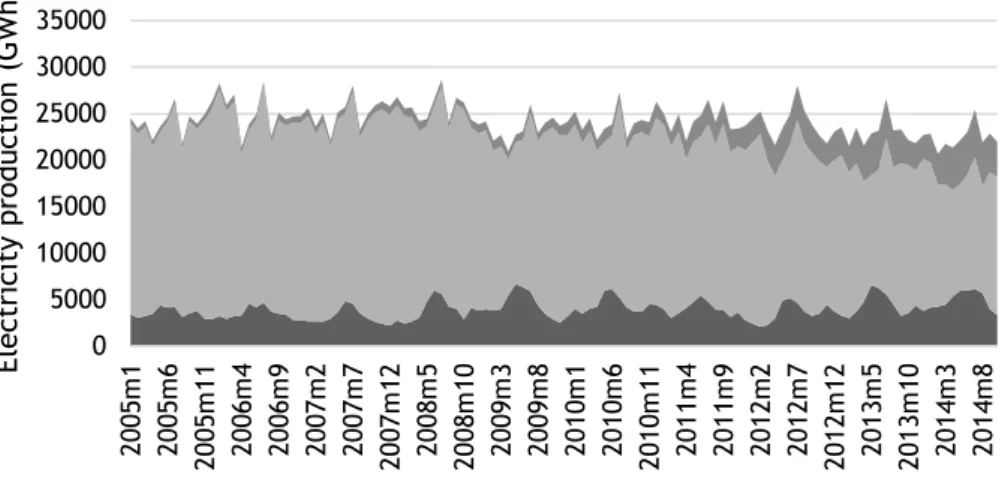
The electricity mix in Italy is using both conventional and renewable sources. They are plants powered by coal, fuel oil and natural gas; or multi-fuel power plants with coal and oil or natural gas and oil; gas turbine plants; combined cycle gas turbines (CCGT); hydro power with storage or run of the river; wind power; solar photovoltaic; geothermal and other renewables. Figure 1 discloses the evolution of the use of the generation sources hydro, and fossil and RES aggregately. A decrease in fossil is contemporaneous of a gradual increase of RES. Several factors could being influencing this cut on consumption, such as the energy efficiency achievements and the consequences of the sovereign debt crisis.

6

Figure 1. Electricity generation by sources

Solar PV and wind are complementary sources, such as noted by Monforti et al. (2014). In Italy, an increase of 1 GWh in production of solar and wind power reduces wholesale market price, in 2.3€/MWh and 4.2€/MWh, respectively. However, the same authors Monforti et al. (2014) point out that these savings are far from enough to counterbalance the financing of renewable promotion programs. Economic instruments to incentivize the utilization and development of wind and solar PV sources are feed-in tariffs and green certificates, respectively. For Antonelli and Desideri (2014) these programs are disadvantageous to the production mix and for Italian final consumer, given that these costs are included within the retail consumer price.

0 5000 10000 15000 20000 25000 30000 35000 20 05 m 1 20 05 m 6 20 05 m 11 20 06 m 4 20 06 m 9 20 07 m 2 20 07 m 7 20 07 m 12 20 08 m 5 20 08 m 10 20 09 m 3 20 09 m 8 20 10 m 1 20 10 m 6 20 10 m 11 20 11 m 4 20 11 m 9 20 12 m 2 20 12 m 7 20 12 m 12 20 13 m 5 20 13 m 10 20 14 m 3 20 14 m 8 El ec trici ty pr odu cti on ( GWh)

7

4. Data and method

This section is compounded by two subsections. In the first one the variables used are identified and the research hypotheses are defined. The second subsection is dedicated to explain the method used.

4.1. Variables description and research hypothesis

The data used in this study have a monthly frequency, for the period from January 2005 till October 2014, i.e. 118 observations. The period was chosen in accordance with the data availability for electricity generation by sources. The data for renewable energy sources are available only since January 2005. October 2014 was chosen based on data availability in November 2014. The data from electricity generation by source is available in the European Network of Transmission System Operators for Electricity (ENTSO-E), in section Data-Country Data Packages, the shortest frequency available is monthly. The industry production index was extracted from the EUROSTAT. The industrial production index is used like was used as the economic activity indicator, because the shortest available GDP frequency is quarterly. The IPI is used as an imperfect proxy of GDP, does not include all sectors of the economy (Sari et al. 2008) (Chevallier 2011). Descriptive statistics of the variables are shown in Table 1.

Table 1.Summary statistics.

Descriptive statistics

Variables Obs Mean S. D. Min Max

LIPI 118 4.6266 0.1986 3.9608 4.8941 LHYDRO 118 8.2527 0.2646 7.6516 8.8057 LFOSSIL 118 9.8068 0.1694 9.3445 10.1018 LRES 118 7.2453 0.6945 6.2265 8.5339 LRXM 118 -3.1198 0.6303 -4.6463 -1.3018 LPUMP 118 5.9468 0.5978 4.6051 6.8533

Note: All variables are in natural logarithms. The variable RXM is the ration between electricity exports and imports. Considering that Italy is a net importer, then the ratio is less than one and as such the logarithm is negative.

The sources of electricity generation we considered are hydropower, fossil fuels, renewable energy sources (without hydroelectric) and system management variables are rate of coverage of imports by exports and pumping systems. The hydropower (LHYDRO) includes the energy generated by stored water and run of the river (mini-hydro). The fossil fuels (LFOSSIL) include electricity generation by hard coal, oil, gas and mixed fuels. The renewable energy sources (LRES) (excluding hydro), are also called new renewables and include wind power, solar

8

photovoltaic, biomass and geothermal. The other variables used are the adjustment variables of the system. The rate of coverage of electricity imports by electricity exports (LRXM) was computed by dividing exports by imports. The electricity consumption in water pumping systems (LPUMP) allows store the generated electricity that cannot be brought into external markets.

The mainstream literature focused on the nexus is looking for empirical evidence for the four traditional hypothesis described above, namely neutrality hypothesis, conservation hypothesis, feedback hypothesis and growth hypothesis. This study goes beyond that traditional approach, analyzing not only the relationship between energy consumption and economic growth, but also analyzing the nature of the relationships between the several electricity sources which constitutes the electricity mix in Italy. As such, in addition to test those traditional hypothesis, five new research hypothesis regarding the relationships between the electricity sources were defined, as follows.

 H1 - On contrary to the fossil sources, the RES are not stimulating economic growth.

Some of the recent literature has not confirmed the positive effect of new renewable sources in economic growth. For instance, (Marques et al. 2014) analyzing the Greek economy concludes that the renewables are not causing economic growth. Given that Italy is under the influence of common objectives defined within the EU concerning the RES targets, then it is anticipated that fossil sources stimulate economic growth, unlike renewable sources.

 H2 - The development of RES requires higher levels of income.

The development of renewable electricity sources is associated with large investment, given that they are capital intensive. These investments are associated in the literature with countries with higher levels of wealth. This appears be a necessary condition that enables the countries to accommodate this effort to diversify sources, thus avoiding reflect on consumers by increased tariffs. Ultimately, this prevent the economy, as a whole, from having to bear the high development costs of these investments in renewables.

 H3 - The increasing penetration of RES into the electricity mix causes a substitution effect of the fossil sources.

As larger is the use of renewable sources, then it is expected that there is replacement of fossil fuels already installed. Indeed, assuming that the demand is not affected by the additional use of renewable sources, then the larger the use of RES, the lower the use of fossil sources will be.

9

The hydropower allows the storage of water in order differ in time the generation of electricity and as such, even so renewable, it is not a source with identical intermittency characteristics such as wind and solar PV. Besides its long tradition in generating electricity, the recent technology developments make it capable of turn on quickly. This fact is more evident on the run-of-the river hydropower plants, which are usually coupled with the pumping.

 H5- -The RES provokes electricity exports.

Attending to the intermittency in the generation of the renewables, it is expected that at some periods of a day those coincident with great availability of resource, including wind, may lead to oversupply. Thus, keeping the demand unchanged, it is expected that this excess of electricity could be used to export or, alternatively, to pump water storage.

4.2. Method

The Italian electric power system is strongly managed and therefore presupposes the existence of endogeneity between the variables. There are models, VAR/VECM, that are used specifically to approach this type of questions. The ARDL model (Shin et al. 1992) is another type of structure relatively robust, but with different assumptions. This structure allows different integration order of variables, provided they are not I(2), also allows different independent variables, different lag-lengths within the model and it is less restrictive. The ARDL model is particularly useful, allows to observe separately short- and long-run effects.

To examine the properties of stationary traditional tests are made. Traditional tests are ADF (Augmented Dickey-Fuller test), PP (Phillips-Perron test) (Phillips and Perron 1988) and KPSS (Kwiatkowski-Phillips-Schmidt-Shin test) (Shin et al. 1992). These test may show inappropriate results, due to the existence of structural breaks in the time series. Due to the characteristics of the variables and the monthly frequency of the data the system is subject to shocks To overcome this potential problem the unit root test with structural break Zivot and Andrews (1992) and Perron (1989) are made.

Different order of integration of the variables were detected, the implementation of causality developed by Toda and Yamamoto (1995) was made. This econometric technique can be used independently of the stationarity proprieties of the variables. This procedure is based on a WALD test in a VAR model in level (Bruns and Gross 2013). Toda-Yamamoto causality is a mixed analysis short- and long-run.

10

t t it i i t

L

q

x

z

y

p

L









(

,

)



(

,

)



'



(1)

where L is the lag operator; ∅(𝐿, 𝑝) = 1 − ∅𝐿 − ∅2𝐿2− ∅3𝐿3− ⋯ − ∅𝑝𝐿𝑝 and 𝛽𝑖(𝐿, 𝑞𝑖) = 𝛽𝑖0+ 𝛽𝑖1𝐿 + 𝛽𝑖2𝐿2+ ⋯ + 𝛽𝑖𝑞𝐿𝑞𝑖 and z is a vector of deterministic variables including the constant, trend and exogenous variables with fixed lags, p and qi are the lag lengths,



'

represents coefficient on the deterministic variables, and



is a error term. ytis the dependent variable and

x

it _{represents explanatory variables. The error correction model is shown in equation 2.}

An equation (2) for all variables was estimated,







 

                   k i p j k i i q j ij it j t t j t j t it i t x z y x p ECT y 1 1 ˆ 1 1 1 ˆ 1 , 1 * * 0 '   (1,ˆ)   (2)

where _{is the first difference operator, the ECT (error-correction term) is given by}

    _

_

_  k i i it t t x z y 1 ' ˆ ˆ



and  



 p i p q 1 1 ) ˆ , (  

measure the quantitative significance of the error correction term. The coefficients

* j



and * ij



relate to the short-run dynamics of the model’s convergence to equilibrium. The long memory of the variables is characterized by statically significant ECT, there is a certain adjustment speed between the variables for the model converge to equilibrium.

Diagnostic residual test were made, namely ARCH test for heteroscedasticity; Breusch-Godfrey serial correlation LM test; Jarque-Bera normality test and stability coefficients test of CUSUM and CUSUM of squares.

11

5. Results

5.1. Unit root tests

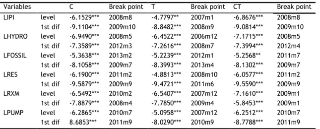
The null hypothesis for the ADF test and PP test is: the variable has a unit root, i.e., the variable is non-stationary. On contrary to ADF and PP, the KPSS test has the null hypothesis, of stationarity. This tests reveals no consensus about the integration order of the series. These tests can be seen in Table 7 the appendix. In some cases, they appear be borderline I(0)/I(1). Notwithstanding, the tests assure that variables are not I(2). To make sure that the variables are not I(2), additional unit root tests with structural breaks were carried out Zivot and Andrews (1992) (Table 2) and Perron (1989) (Table 8). For both tests the null hypothesis is that the variable has a unit root with structural break. The tests corroborate that the variables are not definitely I(2).

Table 2. Unit root tests with structural breaks Zivot-Andrews

Variables C Break point T Break point CT Break point

LIPI level -6.1529*** 2008m8 -4.7797** 2007m1 -6.8676*** 2008m8 1st dif -9.1104*** 2009m10 -8.8482*** 2008m9 -9.0814*** 2009m10 LHYDRO level -6.9490*** 2008m5 -6.4522*** 2006m12 -7.1715*** 2008m5 1st dif -7.3589*** 2012m3 -7.2616*** 2008m7 -7.3994*** 2012m4 LFOSSIL level -5.3638*** 2013m2 -5.2239*** 2012m1 -5.2568** 2011m7 1st dif -8.1058*** 2009m7 -8.3993*** 2013m4 -8.1302*** 2009m7 LRES level -6.1900*** 2011m2 -4.8813*** 2008m10 -6.0577*** 2011m2 1st dif -9.5879*** 2009m9 -9.4721*** 2011m6 -9.5590*** 2009m9 LRXM level -6.5492*** 2010m2 -6.5407*** 2007m12 -7.1610*** 2009m1 1st dif -7.8879*** 2008m4 -7.7850*** 2009m4 -5.8453*** 2009m1 LPUMP level -6.2865*** 2010m7 -5.0958*** 2007m12 -6.2512*** 2010m7 1st dif 8.6853*** 2011m9 -8.0290*** 2010m9 -8.7788*** 2011m9 Notes: C stands constant; T stands trend; CT stands constant and trend; ***, ** and * represents significant level for 1%, 5% and 10%, respectively

5.2. Toda-Yamamoto causality test

The Toda-Yamamoto procedure can be observed on Table 3. The variable LPUMP was used as exogenous variable, because was not caused by any variable, but causes other variables.

Table 3. Toda-Yamamoto causality test

Dependent Variable

LIPI LHYDRO LFOSSIL LRXM LRES

LIPI does not cause 2.1382 0.8320 7.1845** 5.9427*

LHYDRO does not cause 5.2518* 8.2481** 0.6802 6.5433**

LFOSSIL does not cause 29.3526*** 17.2411*** 0.6850 4.8857*

LRXM does not cause 9.8669*** 2.8805 6.3530** 5.7179*

LRES does not cause 5.7682* 0.5417 1.9582 3.4185

ALL 35.3210*** 29.3143*** 19.0759** 20.5671*** 15.562**

Notes: the results are based on Chi squared statistics.

12

The Toda-Yamamoto approach has desired econometric properties in residual tests. The error term follows normal distribution (Jarque-Bera statistic: 9.2488; p-value: 0.5087). It does not exist serial correlation in first order (LM statistics: 18.6789, p-value: 0.8123) and the errors are homoscedastic (chi squared: 651.6598, p-values: 0.4194).

Globally all variables cause and are caused, so the variables are endogenous. As you can see

LIPI is caused by all variables, LRES also is caused by all variables. LHYDRO is only caused by LFOSSIL at 1% significant level and LRXM is only caused by LIPI.

5.3. ARDL Model

After the verification of the stationary and endogeneity proprieties of the variables, the ARDL model was estimated (Table 4). Five ARDL models were estimated, have as dependent variable electricity generation sources, industrial production index and ratio of coverage of imports by exports, both in first differences. Where the dependent variables are DLIPI, DLHYDRO,

DLFOSSIL, DLRES and DLRXM, that corresponding to the models I, II, III, IV and V, respectively.

Impulse and shift dummies were used to control the outliers and structural breaks identified in Zivot-Andrews unit root tests with structural breaks. The use of these dummy variables should be made as parsimonious as possible.

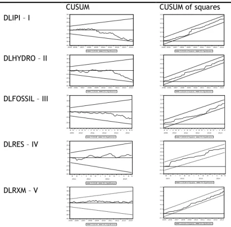
The ARCH test for heteroscedasticity has the null hypothesis: the homoscedasticity. In this test the null hypothesis cannot be rejected, regardless of order test. To the Breusch-Godfray serial correlation LM test the null hypothesis that is no serial correlation, cannot be reject in the first order serial correlation. In the second and third orders also cannot be rejected, except in the model II. Jarque-Bera normality test check the error term follows normal distribution. The coefficients stability test (Figure 1) CUSUM and CUSUM squares (Garbade 1977) suggest the parameters stability for all equations. The tests ensure the quality of the estimates.

13

Table 4. Estimated ARDL

Dependent Variable

I - DIPI II - DLHYDRO III - DLFOSSIL IV - DLRES V - DLRXM constant 5.525989*** 10.5762*** trend 0.0068*** DLIPI 0.2883*** -1.2889*** DLHYDRO 0.3303*** -0.1350*** 0.4637* DLHYDRO(-1) 0.2789*** -0.1396* DLFOSSIL 1.1657*** -0.3253** 2.0731*** DLFOSSIL(-1) -0.5166*** DLRES(-1) -0.1675** DLRXM -0.0950*** 0.0539*** DLRXM(-1) 0.0591*** LIPI(-1) -0.7129*** 0.2973*** -0.2598*** LHYDRO(-1) -0.2693*** -0.4735*** 0.0661*** LFOSSIL(-1) -0.7351*** -0.0560*** 0.1091* LRES(-1) -0.4009*** LRXM(-1) -0.3883*** LPUMP(-1) 0.0910*** Time dummies id2009m7 0.1419* sd2011M06 0.1893*** Diagnostic tests ARS 0.7801 0.3994 0.5028 0.2434 0.3769 SER 0.126264 0.1397 0.0775 0.1273 0.4711 Jarque-Bera 0.125451 0.6975 0.5004 0.1509 0.7589 LM (1) [0.4197] (1) [0.2178] (1) [0.1056] (1) [0.8988] (1) [0.5395] (2) [0.7119] (2) [0.0103] (2) [0.2717] (2) [0.9920] (2) [0.6399] (3) [0.8719] (3) [0.0173] (3) [0.0081] (3) [0.7317] (3) [0.7293] ARCH (1) [0.8089] (1) [0.4526] (1) [0.1924] (1) [0.5586] (1) [0.5475] (2) [0.8490] (2) [0.1810] (2) [0.3626] (2) [0.8301] (2) [0.7453] (3) [0.9239] (3) [0.3226] (3) [0.3457] (3) [0.8351] (3) [0.7902] Notes: diagnostic tests results are based on F-statistics. [ ] represented the p-values of F-statistic and ( ) represented lags for the variables. ARS denoted Adjusted R-squared. SER means standard error of regression. Jarque-Bera is a normality test. LM is Breusch-Godfray serial correlation LM test. ARCH denotes ARCH test for heteroscedasticity.***, ** and * represents significant level for 1%, 5% and 10%, respectively.

For all models the value of Error Correction Mechanism (ECM) is significant at 1% level and have a negative signal. This shows the short adjustment speed for the long term. The ECM is specified by -0.7129, -0.4735, -0.0560, -0.4009 and -0.3883for model I, II, III, IV and V, respectively. Model I shows fast speed of adjustment, while model II, IV and V have a moderate speed of adjustment. The model III reveal a very slowly speed of adjustment.

14

CUSUM CUSUM of squares

DLIPI – I -40 -30 -20 -10 0 10 20 30 40 20052006 2007 2008 20092010 2011 2012 20132014 CUSUM 5% Significance -0.2 0.0 0.2 0.4 0.6 0.8 1.0 1.2 2005 2006 20072008200920102011201220132014 CUSUM of Squares 5% Significance

DLHYDRO – II -40 -30 -20 -10 0 10 20 30 40 20052006 2007 20082009 2010 20112012 20132014 CUSUM 5% Significance -0.2 0.0 0.2 0.4 0.6 0.8 1.0 1.2 2005200620072008200920102011201220132014 CUSUM of Squares 5% Significance

DLFOSSIL – III -30 -20 -10 0 10 20 30

IIIIVIIIIIIIVIIIIIIIVIIIIIIIVIIIIIIIVIIIIII IV 2009 2010 2011 2012 2013 2014 CUSUM 5% Significance -0.2 0.0 0.2 0.4 0.6 0.8 1.0 1.2 1.4

IIIIVIIIIIIIVIIIIIIIVIIIIIIIVIIIIIIIVIIIIII IV 2009 2010 2011 2012 2013 2014

CUSUM of Squares 5% Significance

DLRES – IV -20 -15 -10 -5 0 5 10 15 20

III IV I II III IV I II III IV I II IIIIV 2011 2012 2013 2014 CUSUM 5% Significance -0.4 -0.2 0.0 0.2 0.4 0.6 0.8 1.0 1.2 1.4

III IV I II III IV I II III IV I II IIIIV 2011 2012 2013 2014

CUSUM of Squares 5% Significance

DLRXM – V -40 -30 -20 -10 0 10 20 30 40 20052006 2007200820092010 201120122013 2014 CUSUM 5% Significance -0.2 0.0 0.2 0.4 0.6 0.8 1.0 1.2 2005200620072008200920102011201220132014 CUSUM of Squares 5% Significance

Figure 2. CUSUM and CUSUM of squares tests

The likelihood ratio exclusion has been performed for each the results are exposed in Table 5. The independent variables are statistically significant, consequently should be preserved in the model.

Table 5. Likelihood radio exclusion test Dependent Variable

I - DLIPI II - DLHYDRO III - DLFOSSIL IV - DLRES V - DLRXM

DLIPI 74.10488*** 34.75544*** DLHYDRO 21.53353*** 10.54690*** 3.262830* DLHYDRO(-1) 10.78092*** 2.928153* DLFOSSIL 74.57216*** 5.95496** 16.41294*** DLFOSSIL(-1) 15.59222*** DLRES(-1) 4.202334** DLRXM 20.00912*** 16.77789*** DLRXM(-1) 7.853306*** LIPI(-1) 10.07162*** 25.63578*** LHYDRO(-1) 28.82544*** 10.45958*** LFOSSIL(-1) 27.63731*** 3.559397* LPUMP(-1) 7.567501***

Note: ***, ** and * represents significant level for 1%, 5% and 10%, respectively. Semi-elasticities and elasticities for all models was performed in Table 6.

15

Table 6. Semi-elasticities and elasticities

I - DLIPI II - DLHYDRO III - DLFOSSIL IV - DLRES V - DLRXM

DLIPI 0.2883*** DLHYDRO 0.3303*** -0.1350*** 0.4637* DLHYDRO(-1) 0.2789*** -0.1396* DLFOSSIL 1.1657*** -0.3253** 2.0731*** DLFOSSIL(-1) -0.5166*** DLRES(-1) -0.1675** DLRXM -0.0950*** 0.0539*** DLRXM(-1) 0.0591*** LIPI 0.7417*** -0.6691*** LHYDRO -0.3777*** 1.1796*** LFOSSIL -1.5526*** 0.2722*** LPUMP 0.1923**

***, ** and * represents significant level for 1%, 5% and 10%, respectively.

In the model I an increase of 1% in electricity generation under HYDRO decrease 0.378 % in IPI, in the long-run. On respect to short-run, an increase of 1 percentage point (pp) in DLHYDRO,

DLFOSSIL, and DLRES lagged once and DLRXM has an impact of 0.330, 1.166, -0.167 and 0.095

pp, respectively. The HYDRO model indicates that FOSSIL produces an effect in short- and long-run, 0.279 pp and -1.553 %, respectively. The semi-elasticity of IPI in the model III reveal the positive effect on electricity generation under FOSSIL sources. The HYDRO sources has a different effect in the affectation of the FOSSIL sources, in both short-run (-0.135 pp) and long-run (1.180%).

16

6. Discussion

This work is focused on the analysis of the dynamics of interactions between electricity generation sources, both renewables and renewables. Moreover, the work assess the kind of relationships could be observed between these several sources and the economic activity. The sectorial measure Industrial Production Index is used, given that the GDP was unavailable for the monthly data frequency. This data frequency reveals be appropriate. Indeed, working with annual data would involve an unsatisfactory number of observations, meanwhile the required time span will not allow distinguishes the contribution from each renewable source given that they are very recent. Accordingly, this study only carefully could be confronted with the traditional literature focused on the energy-growth nexus. The ARDL approach used has allowed the analysis of the effects verified both on the short- and on the long-run. Moreover, the results from the Toda-Yamamoto causality test and the ARDL approach reveal great consistency.

There is evidence for the traditional feedback hypothesis for the fossil sources, even so only on the short-run. Actually, there is a causal relationship from fossil to IPI and the vice-versa is also true. However, that relationship is not observable on the long-run. The nature of the effect of the hydropower is dissimilar on the short-, and on the long-run. Regarding the renewables, other than the hydro power, these sources are not stimulating the economic activity, on contrary of fossil sources, which supports the H1. Instead, RES lagged once is hampering economic activity, which is in line with, for instance (Ocal and Aslan 2013). At the meantime, on the long-run the IPI incentives de deployment of renewables, which is also consistent with the literature. Indeed, it seems that greatest wealth of a country will allow enlarge the contribution of renewables. In this way, the analysis provide support for the H2. If renewables require abundance and prosperity, the natural question is that how poorest countries, or countries with budgetary difficulties, such as Italy and other EU countries, can meet the renewables targets? The recent crisis worldwide and particularly that affecting the southern European countries have forced subject some countries to adjustment programs. These programs further hindered the development of the economy, making more difficult the go ahead in the deployment of renewable sources.

As much is common knowledge these goals are not conditional of the level of richness of each country. Accordingly, aggressive strategies to promote renewables in the absence of a strong domestic financial support could provoke undesirable consequences on the prosperity of the country. In fact, this evidence is observed on the negative effect from renewables to IPI, observed in model I, and which is consistent with the noted by (Antonelli and Desideri 2014) about the high prices on consumption. In short, IPI requires larger use of fossil sources on the short-run, given that these sources can be able to enlarge its contribution to the electricity mix

17

almost instantaneously. By its turn, RES are stimulated by IPI only on the long-run. On one hand these sources have not capacity of storage and as such they could not satisfy instantaneously additional demand. On the other hand, the enhancement of the economic activity releases financial resources to invest on renewables. All this evidence constitutes a strong support for a revision of the EU targets, which should be fixed in accordance with the performance of the economic activity.

What has been said ago suggests that the path tracked by renewables is mostly defined by the decision makers. In fact, this autonomous behavior of renewables is also corroborated by the highly statistical significant presence of an increase trend. On the short-run there is indication of a substitution effect between RES and fossil. However, this effect is significant only at 10%. On contrary, on the long-run there is no evidence of substitution effect between these two kinds of sources and as such the H3 is verified only for the short-run. Indeed, more RES require more fossil availability to backing the intermittency of the renewables, which constitutes support for the H4. Regarding the variables external trade and pumping, which are variables of the management of the system, external trade reveal be non-significant on the long-run, but pumping reveals a contribution to generate hydropower in the long-run. On the short-run only the external trade is statistically significant. The H5 is partially verified. This is suggesting that the electricity external trade is being used on the short-run to accommodate RES, by backing them.

18

7. Conclusion

The interactions between electricity sources and the economic activity were studied in Italy, for the time span from January 2005 till October 2014. Italy is confronted with the need to diversify the electricity mix in the medium and long-run, meanwhile is faced on short-run with severe budget constraints which have been made worse by the sovereign debt crisis. The Toda-Yamamoto causality testing and the ARDL approach were carried out, in order to be able to full understand the dynamics of adjustment both on the short- and on the long-run. This study contributes to the literature not only by analyzing a specific European Southern country, but essentially by enriching the analysis of the traditional energy-growth nexus. Indeed, the dynamics of adjustment of the several electricity sources is crucial to full understand the consequences of the diversification of the mix.

The findings of this work confirm the presence of the feedback hypothesis in Italy, but only for the fossil sources and only in the short-run. Moreover, this work brings support for the fact that the deployment of renewables requires capability of a country to bear the renewables’ investment. Indeed, to force countries with financial difficulties to accomplish with exigent renewables targets could further worsen the already weak status of their economies. In this way, the 2020 Climate and Energy Package by EU, seems excessively ambitious for Italy.

19

20

References

ADEBOLA,S.;SHAHBAZ, M.,(2015): Natural gas consumption and economic growth : The role of foreign direct investment , capital formation and trade openness in Malaysia. Renewable

and Sustainable Energy Reviews, 42, 835–845.

ANTONELLI,M.;DESIDERI,U.,(2014): The doping effect of Italian feed-in tariffs on the PV market. Energy Policy, 67, 583–594.

APERGIS, N.;PAYNE, J.E.,(2010): A panel study of nuclear energy consumption and economic growth. Energy Economics, 32(3), 545–549.

APERGIS,N.;PAYNE,J.E.,(2009): Energy consumption and economic growth in Central America: Evidence from a panel cointegration and error correction model. Energy Economics, 31(2), 211–216.

BIGERNA,S.;ANDREA BOLLINO,C.;POLINORI,P.,(2015): Marginal cost and congestion in the Italian

electricity market: An indirect estimation approach. Energy Policy, 1–10.

BROUWER,A.S. ET AL.,(2014): Impacts of large-scale Intermittent Renewable Energy Sources on electricity systems, and how these can be modeled. Renewable and Sustainable Energy

Reviews, 33, 443–466.

BRUNS,S.B.;GROSS,C.,(2013): What if energy time series are not independent? Implications for

energy-GDP causality analysis. Energy Economics, 40, 753–759.

CHANG,T.-H.;HUANG,C.-M.;LEE,M.-C.,(2009): Threshold effect of the economic growth rate on the renewable energy development from a change in energy price: Evidence from OECD countries. Energy Policy, 37(12), 5796–5802.

CHEVALLIER, J.,(2011): A model of carbon price interactions with macroeconomic and energy

dynamics. Energy Economics, 33(6), 1295–1312.

CHU,H.P.;CHANG,T.,(2012): Nuclear energy consumption, oil consumption and economic growth

in G-6 countries: Bootstrap panel causality test. Energy Policy, 48, 762–769.

EUROPEAN COMMISSION,(2001): DIRECTIVE 2001/77/EC OF THE EUROPEAN PARLIAMENT AND OF THE

COUNCIL of 27 September 2001 on the promotion of electricity produced from renewable energy sources in the internal electricity market. Official Journal of the European

Communities, 6.

EUROPEAN COMMISSION,(2003): DIRECTIVE 2003/30/EC OF THE EUROPEAN PARLIAMENT AND OF THE COUNCIL of 8 May 2003 on the promotion of the use of biofuels or other renewable fuels for transport. Official Journal of the European Communities, 4(11), 42–46.

EUROPEAN COMMISSION,(2009): DIRECTIVE 2009/28/EC OF THE EUROPEAN PARLIAMENT AND OF THE COUNCIL of 23 April 2009 on the promotion of the use of energy from renewable sources and amending and subsequently repealing Directives 2001/77/EC and 2003/30/EC.

Official Journal of the European Communities, 16–62.

FLORA,R.;MARQUES,A.C.;FUINHAS,J.A.,(2014): Wind power idle capacity in a panel of European

21

GARBADE,K.,(1977): Two Methods for Examining the Stability of Regression Coefficients. Journal of The American Statistical Association, 72(357), 54–63. Available at:

10.1080/01621459.1977.10479906.

GARRONE,P.;GROPPI,A.,(2012): Siting locally-unwanted facilities: What can be learnt from the location of Italian power plants. Energy Policy, 45, 176–186.

GIANFREDA, A.; GROSSI, L.,(2012): Forecasting Italian electricity zonal prices with exogenous variables. Energy Economics, 34(6), 2228–2239.

HALKOS, G.E.; TZEREMES, N.G.,(2014): The effect of electricity consumption from renewable

sources on countries economic growth levels: Evidence from advanced, emerging and developing economies. Renewable and Sustainable Energy Reviews, 39, 166–173.

HELM,D.,(2014): The European framework for energy and climate policies. Energy Policy, 64, 29–35.

KANELLAKIS, M.; MARTINOPOULOS, G.; ZACHARIADIS, T.,(2013): European energy policy—A review. Energy Policy, 62, 1020–1030.

LUND,P.D. ET AL.,(2015): Review of energy system flexibility measures to enable high levels of

variable renewable electricity. Renewable and Sustainable Energy Reviews, 45, 785–807. MARQUES,A.C.;FUINHAS,J. A.;PIRES MANSO,J.R.,(2010): Motivations driving renewable energy in

European countries: A panel data approach. Energy Policy, 38(11), 6877–6885.

MARQUES,A.C.;FUINHAS,J.A.,(2015): The role of Portuguese electricity generation regimes and

industrial production. Renewable and Sustainable Energy Reviews, 43, 321–330.

MARQUES,A.C.;FUINHAS,J.A.;MENEGAKI,A.N.,(2014): Interactions between electricity generation

sources and economic activity in Greece: A VECM approach. Applied Energy, 132, 34–46. MENEGAKI,A.N.,(2011): Growth and renewable energy in Europe: A random effect model with

evidence for neutrality hypothesis. Energy Economics, 33(2), 257–263.

MENEGAKI,A.N.,(2014): On energy consumption and GDP studies; A meta-analysis of the last two

decades. Renewable and Sustainable Energy Reviews, 29, 31–36.

MONFORTI,F. ET AL.,(2014): Assessing complementarity of wind and solar resources for energy

production in Italy. A Monte Carlo approach. Renewable Energy, 63, 576–586.

OCAL,O.;ASLAN,A.,(2013): Renewable energy consumption–economic growth nexus in Turkey. Renewable and Sustainable Energy Reviews, 28, 494–499.

ODHIAMBO,N.M.,(2009): Energy consumption and economic growth nexus in Tanzania: An ARDL

bounds testing approach. Energy Policy, 37(2), 617–622.

OHLER,A.;FETTERS,I.,(2014): The causal relationship between renewable electricity generation

and GDP growth: A study of energy sources. Energy Economics, 43, 125–139.

OMRI,A.,(2014): An international literature survey on energy-economic growth nexus: Evidence from country-specific studies. Renewable and Sustainable Energy Reviews, 38, 951–959. OZTURK,I.,(2010): A literature survey on energy–growth nexus. Energy Policy, 38(1), 340–349. PERRON,P.,(1989): The Great Crash, the Oil Price Shock, and the Unit Root Hypothesis.

22

PHILLIPS,PETER;PERRON,P.,(1988): Testing for a unit root in time series regression. Biomètrica,

75, 335–346.

SARI, R.; EWING, B.T.; SOYTAS, U.,(2008): The relationship between disaggregate energy

consumption and industrial production in the United States: An ARDL approach. Energy

Economics, 30(5), 2302–2313.

SHIN,Y. ET AL.,(1992): Testing the Null Hypothesis of Stationarity Against the Alternative of a Unit Root : How Sure Are We That Economic Time Series Are Nonstationary? , 54, 159–178. SUN,S.;ANWAR,S.,(2015): Electricity consumption, industrial production, and entrepreneurship

in Singapore. Energy Policy, 77, 70–78.

TODA,H.Y.;YAMAMOTO, T.,(1995): Statistical inference in vector autoregressions with possibly

integrated processes. Journal of Econometrics, 66(1-2), 225–250.

ZIVOT,E.;ANDREWS,D.W.K.,(1992): Further Evidence on the Great Crash, the Oil-Price Shock,