A Thesis specially elaborated for obtaining the Degree of Doctor in Information Science and Technology
By
Engº Alexandre M. C. Passos de Almeida, M.Sc.
codes, SN sequences, PN sequences, DFT, UWB
I would like to thank the Prof. Pedro Silva and Prof. Maria Torres for their guidance on the theory of abstract mathematics. I appreciated our fruitful discussions about the marriage between communications engineering and Group and Number theory. I thank also Prof. Pedro
Sebastião, Prof. Rui Dinis and Prof. Francisco Cercas for their support and suggestions in the final revision of this thesis.
Presidente: Doutor Francisco António Bucho Cercas,Prof. Catedrático do ISCTE-IUL Vogais:
Doutor Rui Miguel Henriques Dias Morgado Dinis,Prof. Associado com Agregação da FCT-UNL Doutor Paulo Miguel de Araújo Borges Montezuma de Carvalho,Prof. Auxiliar da FCT-UNL Doutor Marco Alexandre Cravo Gomes,Prof. Auxiliar da Universidade de Coimbra
Doutor Nuno Manuel Branco Souto,Prof. Auxiliar do ISCTE-IUL Doutor Pedro Joaquim Amaro Sebastião,Prof. Auxiliar do ISCTE-IUL
This thesis deals with the design of a class of cyclic codes inspired by TCH codewords. Since TCH codes are linked to finite fields the fundamental concepts and facts about abstract algebra, namely group theory and number theory, constitute the first part of the thesis.
By exploring group geometric properties and identifying an equivalence between some op-erations on codes and the symmetries of the dihedral group we were able to simplify the gen-eration of codewords thus saving on the necessary number of computations. Moreover, we also presented an algebraic method to obtain binary generalized TCH codewords of length N = 2k,k = 1,2,...,16. By exploring Zech logarithm’s properties as well as a group
theo-retic isomorphism we developed a method that is both faster and less complex than what was proposed before. In addition, it is valid for all relevant cases relating the codeword length N and not only those resulting from N = pi 1 for Fermat primes pi. The method also derives the
maximum set of all the codewords of a certain code bringing clear advantages in terms of code size and minimum distance.
In a further investigation we proposed a new generating procedure focusing mostly on group permutations as an efficient way to generate all codewords of a particular cyclic code. For bi-nary sequences associated to sub-Pythagorean primes this method only requires the repeated application of 3 permutations (two for the time domain and one extra for the frequency do-main) and a DFT operation, thus saving memory space and processing time. For general M-ary sequences the procedure may require, at most, M additional permutations.
The performance under a Rayleigh fading channel and the application of these sequences to a variety of communications systems, namely UltraWideband (UWB) and Direct Sequence -Code Division Multi Access (DS-CDMA), were also presented.
As a consequence of our sequence design we can summarize some of the advantages ob-tained: the sequence period or codeword length is not limited to a power of two (and not re-stricted to a Fermat prime minus 1); using the same generating procedure we can produce (both in time and frequency domains) a larger number of codewords resulting in better data rates and/or better error correction; the mathematical knowledge of the code structure permits not having a loose collection of codewords, but a codeword list with a cohesive structure opening up a lot of improvements in terms of coding/decoding steps; the generation procedure is not limited to binary but allows M-ary sequences as well.
Esta tese aborda o projeto de uma classe de códigos cíclicos inspirados nas palavras do código TCH. Os conceitos fundamentais e fatos sobre álgebra abstrata, ou seja, teoria de grupos e teoria dos números, constituem a primeira parte da tese.
Ao explorar as propriedades geométricas dos grupos e a identificação de uma equivalência entre algumas operações sobre as palavras de código e as simetrias do grupo diedral simplificou-se a geração de palavras de código, economizando no número de cálculos necessários. Além disso, desenvolveu-se um método algébrico para obter palavras binárias generalizadas (do tipo TCH) de comprimento N = 2k,k = 1,2,...,16. Ao explorar as propriedades dos logaritmos de
Zech, bem como um determinado isomorfismo desenvolveu-se um método que é mais rápido e menos complexo do que o que foi proposto anteriormente. Além disso, o método é válido para todos os casos relevantes relativos à palavra de código de comprimento N e não só as resultantes de N = pi 1 para primos de Fermat pi. O método também deriva o conjunto máximo de todas
as palavras de um determinado código trazendo vantagens claras em termos de tamanho do código e distância mínima.
Numa investigação mais aprofundada propôs-se um novo procedimento de geração, focal-izado principalmente em grupos de permutações, permitindo uma forma eficiente de gerar todas as sequências de um código cíclico particular. Para sequências binárias associados a primos sub-pitagóricos este método requer apenas a aplicação repetida de 3 permutações (duas para o domínio do tempo e uma extra para o domínio da frequência) e uma operação de DFT, poupando assim espaço de memória e tempo de processamento. Para sequências M-árias mais gerais o procedimento pode exigir, no máximo, M permutações adicionais.
Nesta tese apresentaram-se também exemplos de aplicação destas sequências no contexto de sistemas de comunicação, como por exemplo, UWB e DS-CDMA.
Pode-se resumir algumas das vantagens resultantes do trabalho apresentado:
• o período da sequência (ou comprimento da palavra de código) não é limitada a uma potência de dois (e o seu valor não fica restrito a um primo de Fermat menos uma unidade),
• utilizando o mesmo procedimento de geração pode-se produzir um maior número de palavras de código, resultando em melhores rácios de transmissão de dados e/ou melhorar a capacidade de correcção de erros,
• o conhecimento matemático da estrutura do código permite passar de um conjunto disperso de palavras de código para uma lista de palavras com uma estrutura coesa abrindo uma série de melhorias em termos de codificação/decodificação,
• o procedimento de geração não é limitado às palavras binárias, mas permite sequências M-árias também.
(a1,a2, . . . ,ak) cycle of length k
[E : F] dimension of a field extension of E over F [G : H] index of a subgroup H in a group G cisq cosq + j sinq
deg p(x) degree of p(x) di j Kronecker delta
dimV dimension of a vector space V
/0 the empty set
gcd(m,n) greatest common divisor of m and n. Alternatively represented also as (m,n) hai cyclic subgroup generated by a
A \ B intersection of sets A and B A [ B union of sets A and B a 2 A a is in the set A a b a preceeds b
A \ B difference between sets A and B A ⇢ B A is a subset of B
A ⇥ B Cartesian product of sets A and B a _ b join of a and b
a ^ b meet of a and b
A0 complement of the set A
An A ⇥ ··· ⇥ A (n times)
An alternating group on n letters
ai j the (i,j) element of the matrix A
dmin minimum (Hamming) distance of a code F⇤ multiplicative group of a field F
f 1 inverse of the function f
G ⇠= H G is isomorphic to H G(E/F) Galois group of E over F G/N factor group of G mod N ig ig(x) = gxg 1
id identity mapping m | n m divides n
R[x] ring of polynomials over R Sn symmetric group on n letters
U V direct sum of vector spaces U and V U(n) group of units in Zn
w(x) weight ofx
Z(G) center of a group G
C the set of complex numbers N the set of natural numbers Q the set of rational numbers R the set of real numbers Z the set of integers Zn the integers modulo n
Aut(G) automorphism group of G GF(pn) Galois field of order pn a a primitive element Fp The finite field of order p
lcm(m,n) least common multiple of m and n a ⌘ b mod n a is congruent to b modulo n
Eb Bit Energy
N0 Spectral Noise Density
Rc Code Rate
Z(x) The Zech logarithm of x. Acronyms
AWGN Additive White Gaussian Noise BER Bit Error Rate
CRC Cyclic Redundancy Check DFT Discrete Fourier Transform DS-SS Direct Sequence Spread Spectrum ESD Energy Spectral Density
FDMA Frequency Division Multiple Access FEC Forward Error Correction
FFT Fast Fourier Transform
FH Frequency Hopping
FH-CDMA Frequency Hopping Code Division Multiple Access FH-SS Frequency Hopping Spread Spectrum
HD Hard Decision
IDFT Inverse Discrete Fourier Transform IFF (or iff) If and only if
IFFT Inverse Fast Fourier Transform LoS Line of Sight
LSE Least Square Error
MB-OFDM Multi Band Orthogonal Frequency Division Multiplexing MC-CDMA Multi Carrier Code Division Multiple Access
MUI Multi User Interference NLoS Non Line of Sight
OFDM Orthogonal Frequency Division Multiplexing ORD (ord) Order of an element
PAM Pulse Amplitude Modulation PDF Probability Density Function
PN Pseudo Noise
PPM Pulse Position Modulation
QAM Quadrature Amplitude Modulation PSD Power Spectral Density
Rc The code rate, k/n
RS Reed-Solomon
QPSK Quadrature Phase Shift Keying
SD Soft Decision
SN Sidel’nikov
SNR Signal to Noise Ratio TCH Tomlinson, Cercas, Hughes
List of Figures xv
List of Tables xix
Chapter 1. Introduction 1 1.1. Context 1 1.2. Motivation 3 1.3. Objectives 6 1.4. Thesis overview 6 1.5. Thesis contributions 7
Chapter 2. Algebraic preliminaries 9
2.1. Introduction 9
2.2. Preliminary definitions 9
2.3. Sets and Equivalence Relations 10
2.4. Properties of integers 17
2.5. The Integers mod n and Symmetries 19
2.6. Groups 24
2.7. Prime residue groups 29
2.8. Cyclic Groups 34
2.9. The multiplicative group of complex numbers 36
2.10. Conclusion 38
Chapter 3. Fundamentals of Coding and Number Theory 39
3.1. Introduction 39
3.2. Error-Detecting and Correcting Codes 39
3.4. Some common sequences 56
3.5. Rings and Fields 59
3.6. Introduction to TCH sequences 61
3.7. Conclusion 65
Chapter 4. Generalized TCH via Zech logs 67
4.1. Introduction 67
4.2. Discrete logarithms 67
4.3. Zech logarithm 68
4.4. Equivalent form of standard TCH 74
4.5. Generalized TCH codewords 75
4.6. Codewords for other lengths 81
4.7. Conclusion 86
Chapter 5. Permutations of Sidel’nikov sequences 89
5.1. Introduction 89
5.2. Permutations among TCH codewords 90
5.3. Permutations of Zp 1 91
5.4. Extension to generalized TCH codes 95
5.5. Useful isomorphisms 95
5.6. Sequences associated to partitions of F⇤p 96
5.7. Application to Sidel’nikov sequences 100
5.8. TCH codewords are a subset of SN sequences 101
5.9. Demonstration examples 102
5.10. Extension to q = pn 105
5.11. Sequence detector 107
5.12. Conclusion 108
Chapter 6. Application of sequences to communications 111
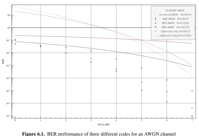
6.1. Code performance results 111
6.2. Synchronization 114
6.3. Channel estimation 131
6.4. Joint coding and spreading in UWB 137
Chapter 7. Conclusion 151
7.1. Synopsis 152
7.2. Future work 153
A.1. Permutation Groups 159
A.2. Dihedral Groups 165
Chapter B. Linear codes 167
B.1. Codes as Groups 167
2.1 Mappings and relations 13
2.2 Composition of maps [1] 14
2.3 Rigid motions of a rectangle 22
2.4 Symmetries of a triangle 23
2.5 Cycle graph of M15 30
2.6 Isomorphic cycle graphs, M15 ' M16 31
2.7 Subgroups of S3 35
2.8 8th roots of unity 38
3.1 Encoding and decoding messages 40
3.2 Binary symmetric channel 43
3.3 Types of rings 60
4.1 Relations between polar integers, i.e. x and the mappings fi(x) 72
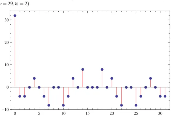
4.2 The autocorrelation of generalized codeword 6F04CEB416 resulting from
(p = 29,a = 2). 77
4.3 The autocorrelation of a codeword from TCH(32,7,5) 77
4.4 The cross-correlation between the (prefixed by C16) generalized codewords
C8746F6816from (p = 29,a = 8) and C44978EE16 from (p = 29,a = 3). 79
4.5 Cross-correlation between codewords from TCH(32,7,5) 79
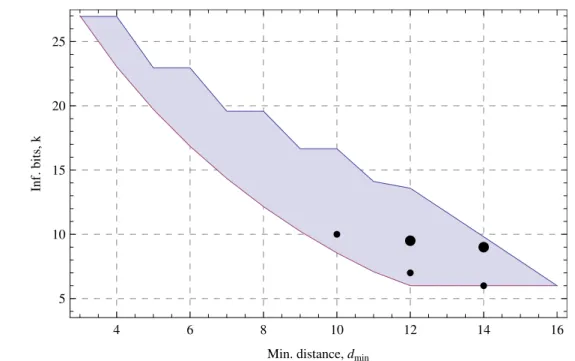
4.6 Comparison between the best 32-bit codes. The smaller points are for the standard TCH and larger points are for the generalized TCH via Zech logarithms. 80
4.7 The autocorrelation of the 64-bit generalized codeword resulting from
(p = 61,a = 10) using a C prefix. 82
4.8 The autocorrelation of a 128-bit generalized codeword. The values for a lag 6= 0 are
within [ 16,24]. 82
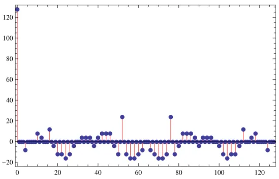
4.9 The crosscorrelation of two 128-bit generalized codewords. All values are within
[ 24,32]. 83
5.1 The circular structure relating all the odd powers of a primitive elementa. In this
case p = 17 anda = 3. 93
5.2 Digraph of all TCH basic codewords for p = 17. Each vertex contains the primitive elementaiand the hexadecimal representation of its associated 16 bit codeword Hai(x).
Using just two permutations, p1 with order 4,p7 with order 2, all f (17 1) = 8
codewords are generated from a single one. 94
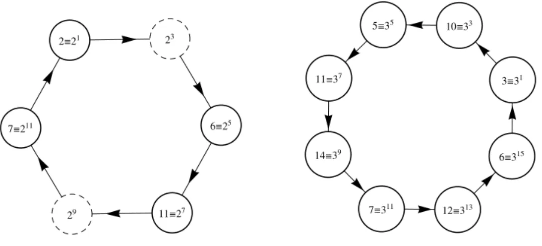
5.3 The circular structure relating the kth powers of a primitive elementa0witha = 2,
p = 13 (left) anda = 3, p = 17 (right). Note that in the figure on the left 3,9 62 M12
while in the figure on the right (corresponding to a Fermat prime case) all odd powers
ofa are primitive elements. 103
5.4 Digraph of all binary SN-sequences for the sub-Pythagorean primes 13 and 17. Each node contains a primitive element ak and the corresponding SN-sequence f
ak(t)
(written in hexadecimal base). The edge labels indicate the permutations used to transform one sequence into another. In the top figure we have the C2⇥C2structure
for p = 13, while in the bottom figure we have the C2⇥C4structure for p = 17. We
consider the initial sequences to be associated with the lowest primitive elements
( f2=0xE25 in the top case and f3=0xD0BC in the bottom case). 104
5.5 Undirected weighted graph where each vertex represents a sub-Pythagorean prime. A vertex p1 is connected to a vertex p2by an edge of weight n = p1+p2 2 such that
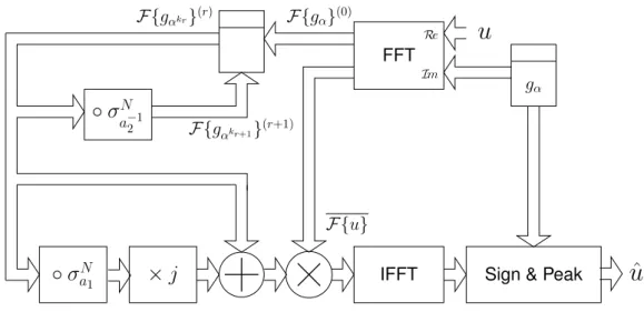
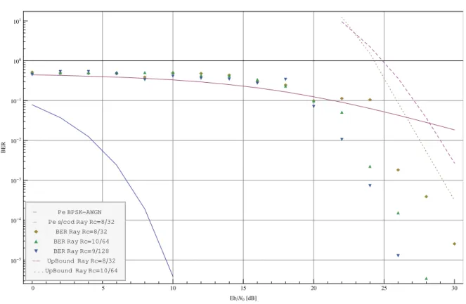
the composite sequence length n is a power of 2 not exceeding 512. Note that in this setting the Fermat primes correspond to the vertices with self-loop edges. 106 5.6 Optimized frequency-based maximum likelihood sequence detector. 108 6.1 BER performance of three different codes for an AWGN channel 113 6.2 BER performance of three different codes for a Rayleigh channel with 0 dB fading 113 6.3 BER performance of three different codes for a Rayleigh channel with -20 dB fading 114 6.4 BER comparison of two 64-bit codes for a Rayleigh channel with 0 dB and -20 dB
6.6 Classical correlation technique 122
6.7 Frequency domain correlation technique 123
6.8 Sequence re-ordering when stored on array x[l,m] 126
6.9 Initial time instant possibilities for synchronization search 127 6.10 Example of a 32 bit sequence partitioned into two 16 bit sub-sequences 128 6.11 Example of a 512 bit data sequence including the sync codes 129 6.12 Probability of making an error in the estimation of the code delay for a misalignment
between the local and received code sequence. 129
6.13 Probability of making an incorrect estimation of the code delay for a misalignment between the local and received code sequence for a single user. 130 6.14 Probability of making an incorrect estimation of the code delay for a misalignment
between the local and received code sequence considering 2 and 4 simultaneous
(asynchronous) users. 131
6.15 Probability of acquisition failure for 16 and 256 chip codes 131
6.16 Block transmission frame format 133
6.17 Signal notation for a) OFDM and b) SC-FDE 134
6.18 Time-domain sequence, absolute value spectrum and scatterplot of a length-256 TCH
code (left column). 137
6.19 A snapshot of the channel frequency response Hk, its estimate eHk using a modified
TCH length-256 code and the corresponding enhanced estimate ˆHk. 138 6.20 A snapshot of the channel impulse response hn, its estimate ˜hn using a spectra
modified TCH length-256 code and the corresponding enhanced estimate ˆhn. 139
6.21 Mean square error of modified-TCH code estimates. 139
6.22 Timing definition for DS and TH transmission schemes. 140
6.23 PSD comparison of a TH-PPM system. 142
6.24 Walsh PSD of the TH-PPM system with TCH codes as hopping codes. 143 6.25 BER results for TH-PPM with TCH codes under a AWGN channel. 145
6.26 TH-PPM with increased number of frames per symbol. 146
6.27 BER results for single-user DS-PAM with TCH codes under a AWGN channel. 146 6.28 Multi-user DS-PAM with TCH 16-chip codes under a AWGN channel. 147
6.29 TH-PPM with 16 chip time-hopping TCH codes using a rake receiver with 8 fingers
and considering a LOS (CM1) and a NLOS (CM2) channel model. 148
6.30 DS-PAM with 16 chip TCH spreading code using a partial rake receiver with 8 fingers
and considering both LOS and NLOS UWB channel models. 148
6.31 CS-TCH for UWB channels using a joint spreading and coding operation. 149
7.1 All the Sidel’nikov codewords from GF(17). 153
A.1 A regular n-gon 165
A.2 Rotations and reflections of a regular n-gon 165
2.1 Multiplication table for Z8 20
2.2 Symmetries of an equilateral triangle 24
2.3 Cayley table for (Z5, +) 25
2.4 Multiplication table for M8 26
2.5 Addition table for Z2⇥ Z2 28
3.1 A repetition code 42
3.2 Distances between 4-bit codewords 46
3.3 Hamming distances for an error-correcting code 47
3.4 Residues modulo 17 53
3.5 DFT transform rules 56
3.6 Verifyinga = 3 as a primitive element of GF(17). 63
3.7 Determination of Kifor (p = 17,a = 3). 64
4.1 Composition of maps corresponding to fi fj(x) 72
4.2 Relationship with the dihedral group D3of order 6 73
4.3 All the values of fi(x) and Z ( fi(x)) for p = 17, x = 0,1,··· , p 2. 73
4.4 Zech values, Z (x) for odd x up to p 2 using the smallest correspondent primitive
elementa 75
4.5 All primitive elements of GF (29) are a subset of the nonresidues given by the
Legendre symbol. 77
4.7 The best generalized 32-bit TCH codewords via Zech logarithms in GF (31). 80 4.8 The best generalized 64-bit TCH codewords via Zech logarithms in GF (53) with
codeword prefixes from GF (13). 81
5.1 Two solutions of equation (5.1) fora = 3 and b = 5. 90
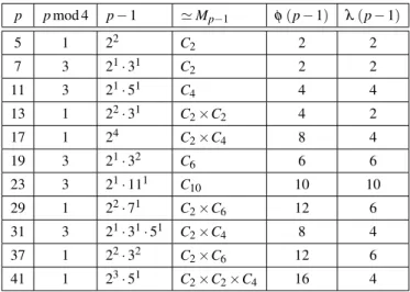
5.2 Isomorphisms between prime residue groups and the direct product of cyclic
subgroups, for the first few primes. 96
5.3 Generators a1 and a2 for permutations of order 2 andl (p 1), respectively. The
value ai 1corresponds to the modular multiplicative inverse of ai. 99
6.1 Sample re-arrangement of a matrix interleaver (of depth NR) 127
7.1 Cycle period for each bit on a 16-bit word upon application of permutationp5. 154
7.2 Cycle period patterns (at level 0) for each bit on a 256-bit word upon application of
permutationp5. 154
7.3 Cycle period patterns for 256-bit words (at level 1). 154
7.4 Cycle period patterns for 256-bit words (at level 2). 154
7.5 Cycle periods (multiplied by 16) of 16-bit words 155
7.6 Alignment of cycle periods between the 16-bit word and the 256-bit word. 155 7.7 The first 256-bit codewords from GF(257) illustrating the embedding of the 16-bit
codewords from GF(17). 156
B.1 Cosets of C 172
INTRODUCTION
1.1. Context
The basic model for communication has remained unchanged for several decades, with the central role being played by the newspaper, the telephone and television. As a society, we are shifting our usage of technology from the management and distribution of information towards the creation of symbolic social linkages. Communication is becoming an end in itself, rather than a means for handling information.
The planetary hypermedia available today offers a world each time more flexible and ac-cessible to an individual taking advantage of the privilege of weight absence, ubiquity and interactivity. Moreover the data transfer still uses text, sound and image, but now in a com-plete imbricate manner. The new media is no longer the mass media. We have moved from the broadcast to the point-cast and this brings the self-centered, portable or mobile context to most communication devices. What was previously described as the information technology is now better described as the information and communication technology.
The widespread introduction of the Internet in the 90’s has spawned many innovations and services that stem from its interactive character. The process of adding mobility to interactivity transformed the role of the Internet and other forms of communication and paved the way for yet another set of innovations and services. The convergence of computing and communica-tion is a process that has turned phones into smart mobile terminals with powerful multimedia capabilities.
The Global System for Mobile communication (GSM) and its extended version, the Digital Communication System (DCS), initially developed for Europe has been adopted in more than 80 countries worldwide. The requirements of multimedia applications drove the research for a 3rd generation system, which started around 1990, the significant outcome being the development
of the Universal Mobile Telecommunications System (UMTS). Currently, the evolution in terms of increasing the capacity and speed using new modulation techniques was made in effect by the 3GPP Long Term Evolution (LTE) that were deployed in the end of 2011. The future is already under development and being marketed as 4G LTE-A (A for Advanced), a standard for wireless communication of high-speed data for mobile smartphones and data terminals.
New generations of wireless mobile radio systems [2] aim to provide flexible data rates (in-cluding high, medium, and low data rates) and a wide variety of applications (like video, data, ranging, localization etc.) to the mobile users while serving as many users as possible. The limited available resources like spectrum and power, however, constraint this goal. In fact, the demand for higher data rate is leading to utilization of wider transmission bandwidth, BW. We went from 200 kHz for GSM, 1.25 MHz for IS-95, and 5 MHz for UMTS to 20 MHz for LTE and projected 100 MHz to LTE-A. As the transmission bandwidth gets wider more challenges we need to face due the characteristics of the wireless channel. Among these challenges we find a) diverse channel multipath (resulting from wave reflections and refraction), with impli-cations in Inter-Symbol Interference (ISI) and fading in the time domain as well as frequency selectivity in the frequency domain, b) time variability of the channel gain and Doppler shift in the frequency domain as a direct result of user mobility, c) the need for resource management to compensate for limitations in spectrum access and power availability. As more and more devices go wireless, future technologies will face spectral crowding and coexistence of wire-less devices will be a major issue. Therefore, considering the limited bandwidth availability, accommodating the demand for higher capacity and data rates is a challenging task, requiring innovative technologies that can coexist with devices operating at various frequency bands.
To address these issues Orthogonal Frequency Division Multiplexing (OFDM) has been proposed as an enabling technology. In OFDM a frequency band is divided into overlapping subcarriers that are orthogonal (when one is at its peak all the others cross zero). Since the BW of each subcarrier is small (much less than the coherence bandwidth of the channel) each subcarrier sees flat fading. This is one advantage of this system. OFDM is however not with-out design issues. Due to the usage of multiple subcarriers it can suffer from high Peak-to-Average Power Ratio (PAPR). Subcarrier orthogonality can be broken by carrier frequency offsets. To overcome deep spectral valleys a strong channel coding is advised. Being similar to OFDM, Single-Carrier with Frequency Domain Equalization (SC-FDE) gathered some in-terest and eventually got extended to SC-FDMA to accommodate multi-user access. It uses SC modulation (typically QPSK or 16QAM), Digital Fourier Transform or DFT-spread orthogonal frequency multiplexing and frequency domain equalization. It is currently adopted for the up-link in 3GPP LTE. To estimate the channel a reference signal composed of a symbol by symbol product of an orthogonal sequence and a pseudo-random sequence is used.
1.2. Motivation
All these aspects involving frequency based equalization, Digital Fourier Transforms (DFT), pseudo-random sequences provide us with the motivation to pursue an investigation into meth-ods of either generalizing or optimizing previously known sequences. In our case we had been using TCH sequences so those binary cyclic sequences were the starting point of the work developed in this thesis.
1.2.1. Sequences and coding. In a communications system we are interested in a reliable and at the same time cost effective way of transmitting data from a source to a receiver. The branch of science dealing with these issues is referred to coding theory and it involves the study of codes and their properties. According to the specific discipline (namely mathematics, information theory, electrical engineering etc.) where codes are studied we find their use in applications like network coding, cryptography, data compression and error correction. These last two applications are perhaps the most known and are also referred as source coding, for data compression, and channel coding, for error detection/correction.
Source encoding deals primarily with removing the redundancy of the data to transmit it more efficiently. This happens, for example, in Zip data compression to make computer files smaller or in facsimile transmission where the use of a run length code removes all superfluous data (like sweeping empty lines) and this way decreasing the transmission bandwidth.
On the other hand, channel encoding tries to add redundancy in a way that makes the data more robust against the channel disturbances. These obstacles to a clean transmission can be dust or scratches in a typical music Compact Disk (CD) or fading and noise in a cellular wireless network. In these instances codes like Reed-Solomon (RS) and Low Density Parity Check (LDPC) are used to add extra bits to the source data in order for the receiver to have more information to decode correctly. One objective of channel coding theory is to find codes which a) transmit quickly, i.e. have a good code ratio, b) have a reasonable size, i.e. have many valid codewords, and c) perform adequately at correcting or at least detecting errors. The performance in these (not mutually exclusive) areas generally involves a trade off. Therefore there are codes that are more appropriate, i.e. optimal, than others according to the specific application to which they are targeted.
A sub-field of coding theory is algebraic coding theory dealing with the expression and re-search in algebraic terms of the properties of the codes. Three common properties are codeword length (or period for cyclic codes), code size (total number of valid codewords) and the mini-mum distance between two valid codewords (e.g. Hamming distance for binary or Lee distance for q-ary alphabet).
The two most researched types of codes are block codes and convolutional codes. In the first type, the encoding of the source data is done in blocks. If the sum of any two codewords is also a valid codeword the the block code is a linear one. Examples include, Reed-Solomon, Golay, Hadamard or Hamming codes [3]. To study these codes in a unified way researchers have found a way to relate parameters of different block codes in a form called code bounds. The lower or upper bounds are the result of exploring the relationship between the code rate and distance. The second type of code, i.e. convolutional, takes the fundamental ideal of representing a codeword by the weighted sum of the source symbols. The output of the encoder uses the states of the convolution encoder to convolve with each input bit. In terms of noise protection, in general, a convolutional code does not perform better than an equivalent block code. What it does offer is a greater simplicity of implementation. The encoding process is usually supported by a simple circuit having state memory and feedback logic (normally XOR gates). The decoding process can be implemented in firmware or software. The Viterbi algorithm [4] and related variants is the most used algorithm in decoding convolutional codes.
Two other concerns of coding theory revolve around designing codes to achieve synchro-nization or to better differentiate users in what is called a Code-Division Multiple Access (CDMA) system. In these applications codewords are also referred as sequences. Codes for synchronization purposes are developed so that a phase shift can be readably be detected or corrected allowing multiple signals to be sent on the same channel using the same codeword. In CDMA applications each user is associated with a different code sequence and by evaluating the correlation between different sequences, as a way to differentiate them, several users can share the same channel at the same time.
1.2.2. UWB applications. The convergence of data, entertainment, and mobile commu-nications within the home has created the need for economical technologies and architectures capable of integrating both legacy and new personal area networks. Ultra wideband (UWB) technology is uniquely qualified to address that requirement and was designed specifically to support high data-rate (hundreds of Mbit/s), short range (up to tens of meters), point-to-point wireless communications. UWB, which is an underlay (or sometimes referred as shared unli-censed) system, coexists with other licensed and unlicensed narrowband systems. The trans-mitted power of UWB devices is controlled by the regulatory agencies, such as the Federal Communications Commission (FCC) in the United States and by the European Conference of Postal and Telecommunications Administrations (CEPT) in Europe, so that narrowband systems are affected from UWB signals only at a negligible level. UWB systems, therefore, are allowed to coexist with other technologies only under stringent power constraints. In spite of this, UWB offers attractive solutions for many wireless communication areas, including wireless personal area networks (WPANs), wireless telemetry and telemedicine, and wireless sensors networks.
With its wide bandwidth, UWB has a potential to offer a capacity much higher than the current narrowband systems for short-range applications.
UWB systems present numerous and unique advantages. First of all it introduces unlicensed usage of an extremely wideband spectrum, as mentioned above. The underlay usage of spectrum greatly increases spectrum efficiency and opens new doors for wireless applications. Excellent time resolution is another key benefit of UWB signals for ranging applications. Due to the extremely short duration of transmitted pulses, sub-decimeter ranging is possible. Robustness against eavesdropping (since UWB signals look like noise) and low power transmission are other benefits of UWB.
UWB has several applications all the way from wireless communications to radar imaging and vehicular radar. The ultra wide bandwidth and hence the wide variety of material tion capabilities allows UWB to be used for radar imaging systems, including ground penetra-tion radars, wall radar imaging, through-wall radar imaging, surveillance systems, and medical imaging. Images within or behind obstructed objects can be obtained with a high resolution using UWB.
Similarly, the possibility of acute time resolution and associated accurate ranging capability of UWB can be used for vehicular radar systems (including collision avoidance, guided parking, etc.). Positioning location and relative positioning capabilities of UWB systems are other great applications that have recently received significant attention.
Last but not least is the wireless communication application, which is arguably the rea-son why UWB became part of the wireless world, including wireless home networking, high-density use in office buildings and business cores, UWB wireless mouse, keyboard, wireless speakers, wireless USB, high-speed Wireless Personal Area Networks (WPAN), wireless sen-sors networks, wireless telemetry, and telemedicine.
1.2.3. State-of-the-Art relating TCH codes. TCH codes were first proposed in [5], and further developed in [6]. The motivation behind the development of TCH codes was to obtain a sort of pseudo-noise codewords with good correlation properties and length equal to a power of two, i.e., 2m. The generation of these codes start with the generation of a single codeword,
named basic-TCH, through an algebric equation. From then on, the code is extended through several ad-hoc methods (search and trial) in order to find other codewords with similar charac-teristics (in terms of weight, minimum distance, correlation properties etc.). The performance of these codes was evaluated under All-White Gaussian Noise channels, both alone as well as concatenated with RS codes (with TCH serving as an inner code and a RS code as the outer code).
There have been some investigation work involving TCH codes in the area of satellite com-munications systems [7, 8], in Ultra-wideband systems [9], in optimization of the bit-mapping
of codewords [10, 11], in synchronization [12, 13, 14], in spread-spectrum applications [15], in turbo-codes schemes [16, 17, 18], and studying the performance in a land mobile satellite channel [19], among others.
In view of the above we have tried to develop an efficient receiver that would address, potentially simultaneously, the synchronization, data decoding and channel estimation using fast algorithms and maintaining the same digital frequency processing structure as much as possible.
1.3. Objectives The main objectives of this thesis are:
To use and evaluate TCH family of codes for UWB, exploiting its circular nature and FFT processing thus shifting signal processing from time to frequency domain.
To extend and generalize TCH codes in order to obtain codewords with length equal to a power of two (besides 16, 256, and 65536 already obtained by a previous method).
To design a receiver, exploiting the algebraic structure of the sequences that correspond to the generalized codewords, using multirate and joint channel decoding and acquisition. A mechanism for data rate adaptation is a very important and desirable characteristic. A receiver may use this mechanism to inform a transmitter of the optimal data rate to increase throughput and/or reduce the frame error rate (FER).
1.4. Thesis overview
In chapter 2 we present and discuss some algebraic facts and core concepts necessary for the theoretical work to be developed in chapters 4 and 5. This includes, sets, relations and mappings, and group theory with emphasis in dihedral and cyclic groups. In chapter 3 we present some background on codes and introduce number theory as a link to finite fields. We then present the generation process behind the development of TCH codes that provided the motivation to pursue further work. In chapter 4 we present a generalized construction of TCH codewords using Zech logarithms. First we use the properties of a dihedral group to reduce by 6 the number of computations for each codeword. Then we generalize the construction of code-words by applying the Zech logarithm to a list of odd integers chosen between 1 and p where p belongs to a specific subclass of primes. For the same codeword length we develop algorithms to obtain one codeword from a different one and for different codeword lengths we develop a permutation matrix to obtain codes with all relevant codewords. In chapter 5 we proceed one step further and generalize the construction of codewords through the use of a small number of permutations. Not only we address the construction in the time domain but we also make it work seamlessly in the frequency domain. This procedure allows for the development of an optimal
frequency domain maximum likelihood receiver that links the theoretical work with practical engineering applications. In addition we extend the construction to address finite fields of order pm. In this way we extend the algebraic generation from binary to M-ary sequences. In the first
part of chapter 6, the applications chapter, we evaluate the performance of the generalized codes presented earlier. We then address the transversal problem of frame synchronization in the con-text of DS-CDMA systems using cyclic sequences and using signal processing methods in the frequency domain. We also briefly address how those sequences are employed in frequency do-main channel estimators. We finish the chapter with the evaluation of a UWB (correlation and multi-rate) receiver proposing to use cyclic sequences for synchronization while also serving to spread and code data.
1.5. Thesis contributions
The core work of this thesis corresponds to the theoretical design of TCH-type codewords or sequences. We provide strong algebraic mechanisms to generate all codewords of a code from a single initial codeword. The construction works both for the time domain as well as for the frequency domain. Moreover we consider not only binary codewords but M-ary codewords and we do not restrict the length of codewords to be p 1 with p a Fermat prime. We consider p to belong in a specific class of primes opening a much greater range of codeword lengths as well as allowing us to explore a specific code structure. A summary of results was published in [20]. The work developed in chapter 4 is presented in [21] and that of chapter 5 in [22].
Another contribution uses an FFT signal processing block where the sequence length is partioned into a product, N = L ·M, with N,L,M positive integers. In the process of obtaining a N-point DFT we make use of M DFT’s with L points each. This signal processing core process data in blocks of N samples rearranging them in such a way that an inherent matrix interleaver is involved. These two features are exploited in CDMA systems for synchronism acquisition (besides the usual data decoding), [12],[23],[24].
The application of TCH codewords in UWB systems was presented in [9].
Another contribution was made by modifying TCH codes in order to use them in frequency domain channel estimators. The spectrum of a basic TCH polynomial was changed by sup-pressing the two zero points at k = 0 and k = N/2. Although this has implications on the code amplitude (for odd samples) it does not alter significantly the code correlation properties.
A brief performance study comparing TCH sequences with the generalized ones, under a channel with Rayleigh fading, is presented in the applications chapter of the thesis.
ALGEBRAIC PRELIMINARIES
2.1. Introduction
In general, a telecommunications engineer does not have a strong background in abstract algebra. It is the purpose of this chapter to introduce the reader to the core material necessary for a deeper understanding of the theory presented in chapters 4 and 5 of this thesis thus making it as much self contained as possible.
To find and study applications of abstract algebra a basic knowledge of set theory, equiva-lence relations, and matrices is a must. Therefore we have organized this chapter as follows. Sections 2.2 to 2.4 present introductory material including set theory, mappings and partitions. Then in section 2.5 we begin the study of algebraic structures by investigating sets associated with single operations that satisfy certain reasonable axioms. From here on we concentrate on group theory. The material presented here is mostly based on [1] but we provide other references for completion.
2.2. Preliminary definitions
In the study of abstract mathematics, we assume some rules about the structure of a collec-tion of objects S . These rules are called axioms. Our objective is to obtain other informacollec-tion about S , using logical arguments and the axioms for S .
DEFINITION 1. A statement in logic or mathematics is an assertion that is either true or false.
That statement is called a proposition if we can prove it to be true. DEFINITION2. A proposition of major importance is called a theorem.
Sometimes we break the proof a theorem into modules, i.e. into several supporting propo-sitions, which are called lemmas, and refer back to these results to prove the main result. If we can prove a proposition or a theorem, it is generally possible to derive other related propositions called corollaries.
2.3. Sets and Equivalence Relations
2.3.1. Set Theory. A well-defined collection of objects is called a set. It’s definition im-plies that we can determine for any given object x whether or not x belongs to the set. If x belong to a set then it is called an element or member of the set. We will denote by capital letters, such as A or X; if a is an element of the set A, we write a 2 A.
Generally, there are two ways to specify a set: by listing all of its elements inside a pair of braces or by stating the property that determines whether or not an object x belongs to the set. Thus, we write
X = {x1,x2, . . . ,xn}
for a set containing elements x1,x2, . . . ,xnor alternatively
X = {x : x satisfies P}, X = {x | given P} if each x in X satisfies a certain property P.
Some of the more important sets that we will consider are the following: N = {n : n is a natural number} = {1,2,3,4,...}; Z = {n : n is an integer} = {..., 2, 1,0,1,2,3,...}; Q = {r : r is a rational number} = {p/q : p,q 2 Z where q 6= 0};
R = {x : x is a real number}; C = {z : z is a complex number}.
We find various relations between sets and can perform operations on sets. A set A is a subset of B, written A ⇢ B or B A, if every element of A is also an element of B. For example,
{3,6,7} ⇢ {2,3,4,5,6,7,8,9} and
N ⇢ Z ⇢ Q ⇢ R ⇢ C.
As expected, every set is a subset of itself. A set B is a proper subset of a set A if B ⇢ A but B 6= A. If A is not a subset of B, we write A 6⇢ B; for example, {2,3,7} 6⇢ {2,4,5,8,9}. Two sets are equal, written A = B, if we can show that A ⇢ B and B ⇢ A.
It is convenient to have a set with no elements in it. This set is called the empty set and is denoted by /0. Note also that the empty set is a subset of every set.
To construct new sets out of old sets, we can perform certain operations: the union A [ B of two sets A and B is defined as
A [ B = {x : x 2 Aor x 2 B}; the intersection of A and B is defined by
A \ B = {x : x 2 Aand x 2 B}.
In the case of more than two sets, the union and the intersection, respectively, of the collection of sets A1, . . .Anare written
n [ i=1 Ai=A1[ ... [ An and n \ i=1 Ai=A1\ ... \ An
When two sets have no elements in common, they are said to be disjoint; for example, if E is the set of even integers and O is the set of odd integers, then E and O are disjoint. Two sets A and B are disjoint exactly when A \ B = /0.
Sometimes we will work within one fixed set U, called the universal set. For any set A ⇢ U, we define the complement of A, denoted by A0, to be the set
A0={x : x 2 Uand x /2 A}.
PROPOSITION3. Let A, B, and C be sets. Then (1) A [ A = A, A \ A = A, and A \ A = /0; (2) A [ /0 = A and A \ /0 = /0; (3) A [ (B [C) = (A [ B) [C and A \ (B \C) = (A \ B) \C; (4) A [ B = B [ A and A \ B = B \ A; (5) A [ (B \C) = (A [ B) \ (A [C); (6) A \ (B [C) = (A \ B) [ (A \C).
THEOREM4. (De Morgan’s Laws) Let A and B be sets. Then (1) (A [ B)0=A0\ B0;
2.3.2. Cartesian Products and Mappings.
DEFINITION 5. Given sets A and B, we can form a set of ordered pairs, i.e. the new set A ⇥ B, called the Cartesian product of A and B. That is,
A ⇥ B = {(a,b) : a 2 Aand b 2 B}.
EXAMPLE. If A = {x,y}, B = {1,2,3}, and C = /0, then A ⇥ B is the set {(x,1),(x,2),(x,3),(y,1),(y,2),(y,3)}
and
A ⇥C = /0.
We define the Cartesian product of n sets to be
A1⇥ ··· ⇥ An={(a1, . . . ,an): ai2 Aifor i = 1,...,n}.
If A = A1 =A2 =··· = An, we often write An for A ⇥ ··· ⇥ A (where A would be written n
times). For example, the set N3consists of all of 3-tuples of natural numbers. Subsets of A ⇥ B
are called relations.
DEFINITION 6. A mapping or function f ⇢ A ⇥ B from a set A to a set B. This is a special type of relation (in which for each element a 2 A there is a unique element b 2 B such that (a,b) 2 f ).
Another way of saying this is that for every element in A, f assigns a unique element in B. We usually write f : A ! B or A! B. Instead of writing down ordered pairs (a,b) 2 A ⇥ B, wef write f (a) = b or f : a 7! b. The set A is the domain of f and
f (A) = { f (a) : a 2 A} ⇢ B
is the range or image of f . We can think of the elements in the function’s domain as input values and the elements in the function’s range as output values.
EXAMPLE. Suppose A = {1,2,3} and B = {a,b,c,d}. In Figure 2.1 we define relations f and g from A to B. The relation f is a mapping, but g is not because 1 2 A is not assigned to a unique element in B; that is, g(1) = a and g(1) = b.
1 2 3 A B a b d c 1 2 3 A B a b d c f: g:
Figure 2.1. Mappings and relations
Given a function f : A ! B, it is often possible to write a list describing what the function does to each specific element in the domain. However, not all functions can be described in this manner. For example, the function f : R ! R that sends each real number to its cube is a mapping that must be described by writing f (x) = x3 or f : x 7! x3. Consider the relation
f : Q ! Z given by f (p/q) = p. We know that 1/2 = 2/4, but is f (1/2) = 1 or 2? This relation cannot be a mapping because it is not well-defined. A relation is well-defined if each element in the domain is assigned to a unique element in the range.
If f : A ! B is a map and the image of f is B, i.e., f (A) = B, then f is said to be onto or surjective. A map is one-to-one or injective if a16= a2 implies f (a1)6= f (a2). Equivalently, a
function is one-to-one if f (a1) = f (a2)implies a1=a2. A bijective map is both one-to-one and
onto.
Given two functions, we can construct a new function by using the range of the first function as the domain of the second function. Let f : A ! B and g : B ! C be mappings. Define a new map, composing f and g :
DEFINITION7. The composition of f and g from A to C, is defined by (g f )(x) = g( f (x)).
EXAMPLE. Consider the functions f : A ! B and g : B ! C that are defined in Figure 2.2(a). The composition of these functions, g f : A ! C, is defined in Figure 2.2(b).
In general, order makes a difference; that is, in most cases f g 6= g f . One example where f g = g f would be for f (x) = x3and g(x) =px.3
A B C A 1 2 3 1 2 3 a b c X Y Z g C X Y Z f g o f (a) (b)
Figure 2.2. Composition of maps [1]
EXAMPLE. A matrix multiplication, a b c d ! x y ! = ax + by cx + dy !
can be given a as map TA: R2! R2by TA(x,y) = (ax + by,cx + dy) for (x,y) in R2and using a
2 ⇥ 2 matrix
A = a b
c d !
.
DEFINITION 8. Maps from Rn to Rm given by matrices are called linear maps or linear transformations.
EXAMPLE. Suppose that S = {1,2,3}. Define a map p : S ! S by p(1) = 2
p(2) = 1 p(3) = 3. This is a bijective map. An alternative way to writep is
1 2 3 p(1) p(2) p(3) ! = 1 2 3 2 1 3 ! .
DEFINITION9. For any set S, a one-to-one and onto mappingp : S ! S is called a permu-tation of S.
(1) The composition of mappings is associative; that is, (h g) f = h (g f );
(2) If f and g are both one-to-one, then the composition g f (which is another mapping) is one-to-one;
(3) If f and g are both onto, then the composition g f is onto; (4) If f and g are bijective, then so is the composition g f .
If S is any set, we will use id to denote the identity mapping from S to itself. Define this map by id(s) = s for all s 2 S.
A map g : B ! A is an inverse mapping of f : A ! B if g f = idAand f g = idB; in other
words, the inverse function of a function simply “undoes” the function. A map is said to be invertible if it has an inverse. We usually write f 1for the inverse of f .
EXAMPLE. The function f (x) = x3has inverse f 1(x) =px .3
EXAMPLE. The natural logarithm and the exponential functions, f (x) = lnx and f 1(x) = ex, are inverses of each other provided that we are careful about choosing domains. Observe
that
f ( f 1(x)) = f (ex) =lnex=x and
f 1(f (x)) = f 1(lnx) = elnx=x whenever composition makes sense.
EXAMPLE. Given the permutation
p = 1 2 3
2 3 1 !
on S = {1,2,3}, it is easy to see that the permutation defined by
p 1= 1 2 3
3 1 2 !
is the inverse ofp. In fact, any bijective mapping possesses an inverse, as we will see in the next theorem.
2.3.3. Equivalence Relations and Partitions. To generalize equality we must introduce the concept of equivalence relations and equivalence classes. An equivalence relation (on a set X) is a relation R ⇢ X ⇥ X such that the following properties are obeyed,
• (x,x) 2 R for all x 2 X (reflexive); • (x,y) 2 R implies (y,x) 2 R (symmetric);
• (x,y) and (y,z) 2 R imply (x,z) 2 R (transitive).
Given an equivalence relation R on a set X, we usually write x ⇠ y instead of (x,y) 2 R. If the equivalence relation already has an associated notation such as =, ⌘, or ⇠=, we will use instead that notation.
EXAMPLE. Let p, q, r, and s be integers, where q and s are nonzero. Define p/q ⇠ r/s if ps = qr. Clearly ⇠ is reflexive and symmetric. To show that it is also transitive, suppose that p/q ⇠ r/s and r/s ⇠ t/u, with q, s, and u all nonzero. Then ps = qr and ru = st. Therefore,
psu = qru = qst. Since s 6= 0, pu = qt. Consequently, p/q ⇠ t/u.
DEFINITION 12. A partition P of a set X is a collection of nonempty sets X1,X2, . . .such
that Xi\ Xj= /0 for i 6= j andSkXk=X.
Let x 2 X and let ⇠ be an equivalence relation on a set X. Then [x] = {y 2 X : y ⇠ x} is called the equivalence class of x. We will see that an equivalence relation gives rise to a partition via equivalence classes. Also, whenever a partition of a set exists, there is some natural underlying equivalence relation:
THEOREM 13. Given an equivalence relation ⇠ on a set X, a partition of X is formed by the equivalence classes of X. Conversely, if P = {Xi} is a partition of a set X, then there is an
equivalence relation on X with equivalence classes Xi.
COROLLARY 14. Two equivalence classes of an equivalence relation are either equal or disjoint.
EXAMPLE. Let r and s be two integers and suppose that n 2 N. We say that r is congruent to s modulo n, or r is congruent to s mod n, if r s is evenly divisible by n; that is, r s = nk for some k 2 Z. In this case we write r ⌘ s (mod n). For example, 41 ⌘ 17 (mod 8) since 41 17 = 24 is divisible by 8. We claim that congruence modulo n forms an equivalence relation of Z. Certainly any integer r is equivalent to itself since r r = 0 is divisible by n.
We will now show that the relation is symmetric. If r ⌘ s (mod n), then r s = (s r) is divisible by n. So s r is divisible by n and s ⌘ r (mod n). Now suppose that r ⌘ s (mod n) and s ⌘ t (mod n). Then there exist integers k and l such that r s = kn and s t = ln. To show transitivity, it is necessary to prove that r t is divisible by n. However,
r t = r s + s t = kn + ln = (k + l)n,
and so r t is divisible by n. If we consider the equivalence relation established by the integers modulo 3, then
[0] = {..., 6, 3,0,3,6,9,...}, [1] = {..., 5, 2,1,4,7,10,...}, [2] = {..., 4, 1,2,5,8,...}.
Notice that [0] [ [1] [ [2] = Z and also that the sets are disjoint. We say that the sets [0], [1], and [2] form a partition of the integers.
The integers modulo n are addressed in more detail in section 2.5 and will become quite useful in discussing various algebraic structures such as groups and rings. For further information about these topics the references [25, 26, 27, 28, 29] are appropriate.
2.4. Properties of integers
In this section we will state some fundamental properties of the integers, including mathe-matical induction and the Fundamental Theorem of Arithmetic.
2.4.1. Mathematical Induction. If we are attempting to verify a statement about some subset S of the positive integers N on a case-by-case basis, this is an impossible task if S is an infinite set. Instead, we give a specific proof for the smallest integer being considered, followed by a generic argument showing that if the statement holds for a given case, then it must also hold for the next case in the sequence.
As an example suppose we wish to show that
1 + 2 + ··· + n = n(n + 1)2 for any natural number n.
The formula is true for n = 1 since
1 =1(1 + 1)
but it is impossible to verify for all natural numbers on a case-by-case basis. To prove the formula true in general, a more generic method is required.
Suppose we have verified the equation for the first n cases, say n = 1, 2, 3, or 4. We can generate the formula for the (n + 1)th case from this knowledge. If we have verified the first n cases, then 1 + 2 + ··· + n + (n + 1) = n(n + 1)2 +n + 1 = n 2+3n + 2 2 = (n + 1)[(n + 1) + 1] 2 .
This is exactly the formula for the (n + 1)th case. This method of proof is known as mathemat-ical induction and we summarize it in the following axiom.
2.4.2. First Principle of Mathematical Induction. Let S(n) be a statement about integers for n 2 N and suppose S(n0)is true for some integer n0. If for all integers k with k n0 S(k)
implies that S(k + 1) is true, then S(n) is true for all integers n greater than n0.
We have an equivalent statement of the Principle of Mathematical Induction that is often very useful:
2.4.3. Second Principle of Mathematical Induction. Let S(n) be a statement about inte-gers for n 2 N and suppose S(n0)is true for some integer n0. If S(n0),S(n0+1),...,S(k) imply
that S(k + 1) for k n0, then the statement S(n) is true for all integers n greater than n0.
A nonempty subset S of Z is well-ordered if S contains a least element. Notice that the set Z is not well-ordered since it does not contain a smallest element. However, the natural numbers are well-ordered.
2.4.4. Principle of Well-Ordering. Every nonempty subset of the natural numbers is well-ordered.
Note that the Principle of Well-Ordering given above is equivalent to the Principle of Mathe-matical Induction.
LEMMA 15. The Principle of Mathematical Induction implies that 1 is the least positive natural number.
PROOF. Let S = {n 2 N : n 1}. Then 1 2 S. Now assume that n 2 S; that is, n 1. Since n+1 1, n+1 2 S; hence, by induction, every natural number is greater than or equal to 1. ⇤
THEOREM 16. The Principle of Mathematical Induction implies that the natural numbers are well-ordered.
Induction can also be very useful in formulating definitions. For instance, there are two ways to define n!, the factorial of a positive integer n.
• The explicit definition: n! = 1 · 2 · 3···(n 1) · n.
• The inductive or recursive definition: 1! = 1 and n! = n(n 1)! for n > 1. 2.5. The Integers mod n and Symmetries
We want to define an operation on a set in a way that will generalize such familiar structures as the integers Z together with the single operation of addition, or invertible 2 ⇥ 2 matrices together with the single operation of matrix multiplication. The integers and the 2 ⇥2 matrices, together with their respective single operations, are examples of algebraic structures known as groups.
Modern group theory1arose from an attempt to find the roots of a polynomial (namely in terms of its coefficients). Groups nowadays play an important role in areas such as coding theory, statistics, and the study of symmetries (with examples in areas of biology, physics and chemistry).
We will address groups in section 2.6 but for now let us introduce some mathematical struc-tures that can be viewed as sets with single operations.
2.5.1. The Integers mod n. In the theory and applications of algebra, the integers mod n have become indispensable. They are used in cryptography, coding theory, and the detection of errors in identification codes. We have already seen that two integers a and b are equivalent mod n if n divides a b. The integers mod n also partition Z into n different equivalence classes; we will denote the set of these equivalence classes by Zn. Consider the integers modulo 12 and the
corresponding partition of the integers:
[0] = {..., 12,0,12,24,...}, [1] = {..., 11,1,13,25,...},
...
[11] = {..., 13, 1,11,23,35,...}.
When no confusion can arise, we will use 0,1,...,11 to indicate the equivalence classes [0],[1],...,[11] respectively. We can do arithmetic on Zn. For two integers a and b, define addition modulo n to 1William Burnside’s [30], first published in 1897 one of the first modern treatments of group theory.
be (a + b) (mod n); that is, the remainder when a + b is divided by n. Similarly, multiplication modulo n is defined as (ab) (mod n), the remainder when ab is divided by n.
EXAMPLE. The following examples illustrate integer arithmetic modulo n:
7 + 4 ⌘ 1 (mod 5) 7 · 3 ⌘ 1 (mod 5)
3 + 5 ⌘ 0 (mod 8) 3 · 5 ⌘ 7 (mod 8)
3 + 4 ⌘ 7 (mod 12) 3 · 4 ⌘ 0 (mod 12).
In particular, notice that it is possible that the product of two nonzero numbers modulo n can be equivalent to 0 modulo n.
Table 2.1. Multiplication table for Z8
· 0 1 2 3 4 5 6 7 0 0 0 0 0 0 0 0 0 1 0 1 2 3 4 5 6 7 2 0 2 4 6 0 2 4 6 3 0 3 6 1 4 7 2 5 4 0 4 0 4 0 4 0 4 5 0 5 2 7 4 1 6 3 6 0 6 4 2 0 6 4 2 7 0 7 6 5 4 3 2 1
EXAMPLE. Most, but not all, of the usual laws of arithmetic hold for addition and mul-tiplication in Zn. For instance, it is not necessarily true that there is a multiplicative inverse.
Consider the multiplication table for Z8in Table 2.1. Notice that 2, 4, and 6 do not have
multi-plicative inverses; that is, for n = 2, 4, or 6, there is no integer k such that kn ⌘ 1 (mod 8). PROPOSITION17. Let Znbe the set of equivalence classes of the integers mod n and a,b,c 2
Zn.
(1) Addition and multiplication are commutative: a + b ⌘ b + a (mod n)
ab ⌘ ba (mod n). (2) Addition and multiplication are associative:
(a + b) + c ⌘ a + (b + c) (mod n) (ab)c ⌘ a(bc) (mod n).
(3) There are both an additive and a multiplicative identity: a + 0 ⌘ a (mod n)
a · 1 ⌘ a (mod n). (4) Multiplication distributes over addition:
a(b + c) ⌘ ab + ac (mod n). (5) For every integer a there is an additive inverse a:
a + ( a) ⌘ 0 (mod n).
(6) Let a be a nonzero integer. Then gcd(a,n) = 1 if and only if there exists a multiplicative inverse b for a (mod n); that is, a nonzero integer b such that
ab ⌘ 1 (mod n).
2.5.2. The Method of Repeated Squares. If we want to compute powers modulo n quickly and efficiently the first thing to notice is that any number a can be written as the sum of distinct powers of 2; that is, we can write
a = 2k1+2k2+··· + 2kn,
where k1<k2<··· < kn. This is just the binary representation of a. For example, the binary
representation of 57 is 111001, since we can write 57 = 20+23+24+25. The laws of exponents
still work in Zn; that is, if b ⌘ ax (mod n) and c ⌘ ay (mod n), then bc ⌘ ax+y (mod n). We
can compute a2k
(mod n) in k multiplications by computing a20 (mod n) a21 (mod n) ... a2k (mod n).
Each step involves squaring the answer obtained in the previous step, dividing by n, and taking the remainder.
The method of repeated squares is a very useful tool for RSA cryptography [31]. To encode and decode messages in a reasonable manner under this scheme, it is necessary to be able to quickly compute large powers of integers mod n.
2.5.3. Symmetries. A symmetry of a geometric figure is a rearrangement of the figure pre-serving the arrangement of its sides and vertices as well as its distances and angles. A map from the plane to itself preserving the symmetry of an object is called a rigid motion. For example,
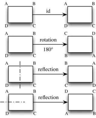
if we look at the rectangle in Figure 2.3, it is easy to see that a rotation of 180 or 360 returns a rectangle in the plane with the same orientation as the original rectangle and the same rela-tionship among the vertices. A reflection of the rectangle across either the vertical axis or the horizontal axis can also be seen to be a symmetry. However, a 90 rotation in either direction cannot be a symmetry unless the rectangle is a square.
A B id D C A B D C A B 180º D C C D B A rotation A B D C B A C D reflection A B D C D C A B reflection
Figure 2.3. Rigid motions of a rectangle
Let us find the symmetries of the equilateral triangle 4ABC. To find a symmetry of 4ABC, we must first examine the permutations of the vertices A, B, and C and then ask if a permutation extends to a symmetry of the triangle. Recall that a permutation of a set S is a one-to-one and onto map i.e. p : S ! S. The three vertices have 3! = 6 permutations, so the triangle has at most six symmetries. To see that there are six permutations, observe there are three different possibilities for the first vertex, and two for the second, and the remaining vertex is determined by the placement of the first two. So we have 3·2·1 = 3! = 6 different arrangements. To denote the permutation of the vertices of an equilateral triangle that sends A to B, B to C, and C to A, we write the array
A B C B C A
! .
Notice that this particular permutation corresponds to the rigid motion of rotating the triangle by 120 in a clockwise direction. In fact, every permutation gives rise to a symmetry of the triangle. All of these symmetries are shown in Figure 2.4.
T T T T T T T T T T T T T T T T T T T T T T T T T T T T T T T T T T T T -A A A A A A B B B B B B C C C C C C B C A B C A A B C C A B C A B A B C reflection reflection reflection rotation rotation identity µ3= ✓ A B C B A C ◆ µ2= ✓ A B C C B A ◆ µ1= ✓ A B C A C B ◆ r2= ✓ A B C C A B ◆ r1= ✓ A B C B C A ◆ id = ✓ A B C A B C ◆
Figure 2.4. Symmetries of a triangle
A natural question to ask is what happens if one motion of the triangle 4ABC is followed by another. Which symmetry isµ1r1; that is, what happens when we do the permutationr1and
then the permutationµ1?2We have
(µ1r1)(A) =µ1(r1(A)) = µ1(B) = C
(µ1r1)(B) =µ1(r1(B)) = µ1(C) = B
(µ1r1)(C) =µ1(r1(C)) = µ1(A) = A.
This is the same symmetry as µ2. Suppose we do these motions in the opposite order,r1then
µ1. It is easy to determine that this is the same as the symmetry µ3; hence,r1µ16= µ1r1. A
multiplication table for the symmetries of an equilateral triangle 4ABC is given in Table 2.2. We will refer to this table in chapter 4.
Notice that in the multiplication table for the symmetries of an equilateral triangle, for every motion of the trianglea there is another motion a0such thataa0=id; that is, for every motion
there is another motion that takes the triangle back to its original orientation.
2Remember that we are composing functions here. Although we usually multiply left to right, we compose
Table 2.2. Symmetries of an equilateral triangle id r1 r2 µ1 µ2 µ3 id id r1 r2 µ1 µ2 µ3 r1 r1 r2 id µ3 µ1 µ2 r2 r2 id r1 µ2 µ3 µ1 µ1 µ1 µ2 µ3 id r1 r2 µ2 µ2 µ3 µ1 r2 id r1 µ3 µ3 µ1 µ2 r1 r2 id 2.6. Groups
The integers mod n and the symmetries of a triangle or a rectangle are both examples of groups. A binary operation or law of composition on a set G is a function G ⇥ G ! G that assigns to each pair (a,b) 2 G a unique element a b, or ab in G, called the composition of a and b. A group (G, ) is a set G together with a law of composition (a,b) 7! a b that satisfies the following axioms.
• The law of composition is associative. That is, (a b) c = a (b c) for a,b,c 2 G.
• There exists an element e 2 G, i.e. the identity element, such that for any element a 2 G e a = a e = a.
• For each element a 2 G, there exists an inverse element a 1in G, such that a a 1=a 1 a = e.
A group G with the property that a b = b a for all a,b 2 G is called abelian or commutative. Groups not satisfying this property are said to be nonabelian or noncommutative.
EXAMPLE. The integers Z = {..., 1,0,1,2,...} form a group under the operation of ad-dition. The binary operation on two integers m,n 2 Z is just their sum. Since the integers under addition already have a well-established notation, we will use the operator + instead of ; that is, we shall write m + n instead of m n. The identity is 0, and the inverse of n 2 Z is written as n instead of n 1. Notice that the integers under addition have the additional property that m + n = n + m and are therefore an abelian group.
Most of the time we will write ab instead of a b; however, if the group already has a natural operation such as addition in the integers, we will use that operation. That is, if we are adding
two integers, we still write m + n, n for the inverse, and 0 for the identity as usual. We also write m n instead of m + ( n).
Table 2.3. Cayley table for (Z5, +)
+ 0 1 2 3 4 0 0 1 2 3 4 1 1 2 3 4 0 2 2 3 4 0 1 3 3 4 0 1 2 4 4 0 1 2 3
It is often convenient to describe a group in terms of an addition or multiplication table. Such a table is called a Cayley table.
EXAMPLE. The integers mod n form a group under addition modulo n. Consider Z5, con-sisting of the equivalence classes of the integers 0, 1, 2, 3, and 4. We define the group operation on Z5 by modular addition. We write the binary operation on the group additively; that is,
we write m + n. The element 0 is the identity of the group and each element in Z5 has an
in-verse. For instance, 2 + 3 = 3 + 2 = 0. Table 2.3 is a Cayley table for Z5. By Proposition 17,
Zn={0,1,...,n 1} is a group under the binary operation of addition mod n.
EXAMPLE. Not every set with a binary operation is a group. For example, if we let modular multiplication be the binary operation on Zn, then Zn fails to be a group. The element 1 acts
as a group identity since 1 · k = k · 1 = k for any k 2 Zn; however, a multiplicative inverse for 0
does not exist since 0 · k = k · 0 = 0 for every k in Zn. Even if we consider the set Zn\ {0}, we
still may not have a group. For instance, let 2 2 Z6. Then 2 has no multiplicative inverse since
0 · 2 = 0 1 · 2 = 2
2 · 2 = 4 3 · 2 = 0
4 · 2 = 2 5 · 2 = 4.
By Proposition 17, every nonzero k does have an inverse in Zn if k is relatively prime to n.
Denote the set of all such nonzero elements in Zn by Mn(sometimes also written U(n)). Then
Mn is a group called the group of units of Zn. Table 2.4 is a Cayley table for the group M8. We
Table 2.4. Multiplication table for M8 · 1 3 5 7 1 1 3 5 7 3 3 1 7 5 5 5 7 1 3 7 7 5 3 1
EXAMPLE. The symmetries of an equilateral triangle described in Section 2.5.3 form a nonabelian group. As we observed, it is not necessarily true thatab = ba for two symmetries a and b. Using Table 2.2, which is a Cayley table for this group, we can easily check that the symmetries of an equilateral triangle are indeed a group. We will denote this group by either S3
or D3, for reasons that will be explained later (section A.2).
EXAMPLE. Let C⇤be the set of nonzero complex numbers. This set C⇤, under the operation of multiplication, forms a group. The identity is 1. If z = a + bi is a nonzero complex number, then
z 1= a bi a2+b2
is the inverse of z. It is easy to see that the remaining group axioms hold.
If a group contains a finite number of elements it is finite, or has finite order; otherwise, the group is said to be infinite or to have infinite order. The order of a finite group is the number of elements that it contains. If G is a group containing n elements, we write |G| = n. The group Z5 is a finite group of order 5; the integers Z form an infinite group under addition, and we
sometimes write |Z| = •.
2.6.1. Basic Properties of Groups.
PROPOSITION18. The identity element in a group G is unique; that is, there exists only one element e 2 G such that eg = ge = g for all g 2 G.
Inverses in a group are also unique. If there were two different inverses g0and g00of an element
g in a group G, then gg0=g0g = e and gg00=g00g = e.
PROPOSITION19. If g is any element in a group G, then the inverse of g, g 1, is unique.
PROPOSITION21. Let G be a group. For any a 2 G, (a 1) 1=a.
PROPOSITION22. If G is a group and a,b,c 2 G, then ba = ca implies b = c and ab = ac implies b = c.
This proposition tells us that the right and left cancellation laws are true in groups. We can use exponential notation for groups just as we do in ordinary algebra. If G is a group and g 2 G, then we define g0=e. For n 2 N, we define
gn=g · g···g | {z } n times and g n=g 1· g 1···g 1 | {z } n times .
THEOREM23. In a group, the usual laws of exponents hold; that is, for all g,h 2 G, (1) gmgn=gm+nfor all m,n 2 Z;
(2) (gm)n=gmn for all m,n 2 Z;
(3) (gh)n= (h 1g 1) nfor all n 2 Z. Furthermore, if G is abelian, then (gh)n=gnhn.
Notice that (gh)n6= gnhnin general, since the group may not be abelian. If the group is Z or Zn, we write the group operation additively and the exponential operation multiplicatively; that
is, we write ng instead of gn. The laws of exponents now become (1) mg + ng = (m + n)g for all m,n 2 Z;
(2) m(ng) = (mn)g for all m,n 2 Z; (3) m(g + h) = mg + mh for all n 2 Z.
It is important to realize that the last statement can be made only because Z and Znare
commu-tative groups.
2.6.2. Subgroups. Sometimes we wish to investigate smaller groups sitting inside a larger group. The set of even integers 2Z = {..., 2,0,2,4,...} is a group under the operation of addition. This smaller group sits naturally inside of the group of integers under addition. We define a subgroup H of a group G to be a subset H of G such that when the group operation of G is restricted to H, H is a group in its own right. Observe that every group G with at least two elements will always have at least two subgroups, the subgroup consisting of the identity element alone and the entire group itself. The subgroup H = {e} of a group G is called the trivial subgroup. A subgroup that is a proper subset of G is called a proper subgroup.
![Figure 4.9. The crosscorrelation of two 128-bit generalized codewords. All values are within [ 24, 32].](https://thumb-eu.123doks.com/thumbv2/123dok_br/18387351.892900/104.892.167.744.151.517/figure-crosscorrelation-bit-generalized-codewords-values.webp)