Nondestructive ultrasonic testing in rod structure with a novel
numerical Laplace based wavelet finite element method
Abstract
Rod structure has been widely used in aerospace engineering and civil engineering. Nondestructive testing is a very important method applied to detect unseen flaws in structures, ultrasonic wave nondestructive testing has been used in many areas. Finite Element Method is one of the most widely used numerical methods but would have a high cost when doing simulation on ultrasonic wave due to the requirement of small time interval and element size. Wavelet based finite element method could improve the spatial resolution with fewer elements needed but still needs very small time interval. Laplace transform could easily convert the time domain into frequency and then inverse to time domain. This paper presents an innovative method combining Laplace transform and B-spline wavelet on interval (BSWI) finite element method, which could not only decrease the element number but also increase the time integration interval. Moreover, this innovative method is applied to simulate the ultrasonic wave propagation in 1D rod structure as well as used for nondestructive testing of damages in rod structures.
Keywords
Ultrasonic wave testing; Wavelet transform; Numerical Laplace transform; B-spine wavelet on interval; Nondestructive Testing
1 INTRODUCTION
During the long time service, structure’s performance may go through being weakened slowly, it also may suffer damages or even being destroyed under serious nature disasters. Thus structure design and nondestructive testing has caught a lot of attention in Aerospace, Mechanical structures and civil engineering, like Zhang et al. (2017b, 2017c), Chen et al. (2015, 2017a, 2017b, 2018), Royston et al. (2011). Structure design is the first step to avoid disaster of happening, and nondestructive testing would help the structure to work safely like Hu and Pratt (2010) and Hu et al. (2016), Park (2015) and Park et al. (2017). Moreover, both experimental and numerical methods have been applied for nondestructive testing, including vibration-based damage detection approaches, like Yam et al. (2003) and Chen et al. (2007), but these methods could not be used for small damages. As more and more engineering problems could be solved and simulated on computer with numerical methods like Hu (2017), Hu et al. (2015), Zhang et al. (2017a), numerical simulation of ultrasonic wave propagation has been studied for a long time. Machine learning has been a hot topic in recent years and has also been used in engineering problems like Liu et al. (2018a, 2018b) and non-destructive testing researches, like Li et al. (2018), Nondestructive testing of
Shuaifang Zhanga Wei Shenb Dongsheng Lib* Xiwen Zhangc Baiyu Chend
a Department of Mechanical Engineering, Penn State University, State College, PA, United States of America. 16803. E-mail: [email protected] b Department of Civil Engineering, Dalian University of Technology, Dalian, Liaoning, P.R. China, 116023. E-mail: [email protected], [email protected]
c Department of Civil Engineering and architecture, University of Jinan, Jinan, Shandong, P.R. China, 250022. E-mail: [email protected]
d College of Engineering, University of California Berkeley, Berkeley, United States of America, 94720. Email: [email protected]
*Corresponding author
http://dx.doi.org/10.1590/1679-78254522
amount of numerical methods have been developed for elastic wave propagation simulation in structures, such as finite element method (FEM) applied by Marfurt (1984) and Moser et al. (1999), finite difference method (FDM) applied by Saenger et al. (2000) and Dai et al. (1995), the spectral element method (SEM) applied by Doyle (1989) and Kudela et al. (2007), boundary element method (BEM) used by Rose (2003) and so on. Obviously, the mesh size and temporal interval could not only determine the accuracy of numerical simulation results, especially due to its high frequency property but also could determine the running time of numerical simulation time. Thus, a good numerical simulation method could not only get accurate results but also could be time efficient.
A lot of numerical models have been developed for numerical simulation of wave propagation in rod structures, like Harari and Turkel (1995), Seemann (1996) and so on. Finite element method is one of the most widely used one and has been applied in simulation of ultrasonic wave propagation by many researchers like Tang and Yu (2017) and Tang et al. (2018), but FEM is mesh dependent to get a accurate enough result, Chen et al. (2012) proposed that at least 10 nodes per wavelength are required to get an accurate simulation results based on the “rule of thumb”. Hence the element size must be very small especially when the frequency of ultrasonic wave is very high. Wavelet finite element method is a relatively new numerical simulation method developed in recent years. Wavelet based finite element method (WFEM) applied by Ma et al. (2003) and Xiang et al. (2007, 2013) is one of the most commonly used method to overcome the shortage of small element size. It should be noticed that there are two kinds of methods are developed based on wavelet transform, the other one method developed by Mitra and Gopalakrishnan (2005) is in frequency domain. This is because wavelet is a good tool for both time and frequency analysis. The B-splined wavelet finite element models used by Chen et al. (2012) should be the most popular ones used by researchers for ultrasonic guided wave propagation in structures. The strongest advantage of time domain WFEM is that only very few elements are needed for accurate analysis. However, the time interval is still required to be very small to find desired solutions, so the cost for calculation is still high.
Another option to solve these problems is to solve the dynamic problems in frequency domain and then convert the solution back to time domain for visualization. FFT based spectral element method is such a method that transforms the governing PDES to a set of ODEs with constant coefficients. Most importantly, usually one single element is sufficient to handle a whole rod structure of any length under the case that there is no discontinuity, so the time cost is much more efficient than traditional FEM. However, due to the assumption of the periodic nature of FFT, FFT based SEM is only applied to solve problems of infinite or semi-finite structures. Igawa et al. (1999) proposed to apply Laplace transform to replace FFT to overcome such problems.
In this paper, a novel method that combines Laplace transform with B-splined WFEM is proposed to simulate the wave propagation in bar structures. This novel Laplace based wavelet finite element method (LWFEM) will combine the advantages of WFEM and Laplace transform, which not only has high spatial resolution with fewer mesh as well as could avoid the periodic assumption of FFT. LWFEM would combine the strength of WFEM which would build a high accurate finite element model with the strength of Laplace transform which will transform the time domain to frequency domain for faster calculation. In such a way LWFEM could be applied in wave propagation as well ultrasonic damage detection with high accuracy and small calculation cost. Numerical simulation of ultrasonic wave propagation in rod structure will be carried out, also the results are compared with other different methods such as traditional FEM, WFEM, SEM. Besides, numerical simulation of damage detection in rod structures will be applied with this novel method.
2. Guided wave propagation in rod and Laplace based WFEM in rod structure
2.1 Ultrasonic guided wave (UGW) propagation and dispersion curves in rod
The governing equations for ultrasonic wave propagation in isotropic structure is shown below based on Navier equations:
2
2
2i i i
i
u
u
f
t
x
(1)where 1 2 3
1 2 3
u u u
x x x
,
is the density of the structure,
,
are Lame constants, f is body force, u is the displacement.Dispersion curves are usually used to depict the relationships between frequency and eigenvalue, as well as phase velocity and group velocity. The relationship between wave velocity and frequency is usually depicted by Pochhammer frequency equation, which is shown in equation (2):
2 2
2 2
2
1 1 0 1 0
2
k J
a J
a
k J
a J
a
4
k
J
a
0
a
(2)Where
2 2
2 2 2
2
,
2,
L T
w
w
k
c
c
𝑤 is frequency,
2
pw
k
c
is the wave number,
J
is the Bessel function.c
L islongitudinal guided wave velocity,
c
T is transverse guided wave velocity,c
p is the phase velocity,
is the lengthof guided waves, 𝑎 is the radius of the rod.
Selecting the appropriate excitation frequency based on the dispersion curves of UGW in rod structure could help excite the ideal UGW mode, so the dispersion curve is really important. A typical dispersion curve for a steel rebar is shown in figure 1 shown in Li et al (2014). The specific procedure of plotting the dispersion curves could be found in Li et al (2014).
Figure 1 Dispersion curves of group velocity.
2.2 B-spline wavelet on interval finite element formulation
B-spline wavelet function is built with piecewise polynomial by joining different knots together on the interval. In order to have at least one inner wavelet on the interval [0 1], for any picked scale j, the dimension of the mth
order B-spline scaling function must satisfy the following equation:
2
j
2
m
1
(3) Wavelet transform would have two corresponding functions, one of which is mother wavelet function (also called wavelet function), and the other is father wavelet function (also called scaling function). 0 scale mth order B-spline scaling function and wavelet function are developed by Goswami et al. (1995). The 0 scale 2nd order scaling functions (j=0, m=2) could be expressed as following,
0 2, 1
1 ,
0,1
0,
else
0 2,0
1
,
0,1
2
,
1,2
0,
else
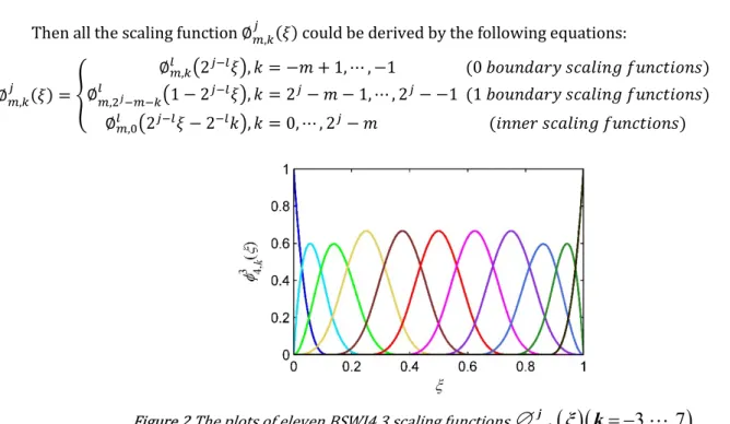
(5)Then all the scaling function ∅ , (𝜉) could be derived by the following equations:
∅ , (𝜉) =
∅ , 2 𝜉 , 𝑘 = −𝑚 + 1, ⋯ , −1 (0 𝑏𝑜𝑢𝑛𝑑𝑎𝑟𝑦 𝑠𝑐𝑎𝑙𝑖𝑛𝑔 𝑓𝑢𝑛𝑐𝑡𝑖𝑜𝑛𝑠)
∅ , 1 − 2 𝜉 , 𝑘 = 2 − 𝑚 − 1, ⋯ , 2 − −1 (1 𝑏𝑜𝑢𝑛𝑑𝑎𝑟𝑦 𝑠𝑐𝑎𝑙𝑖𝑛𝑔 𝑓𝑢𝑛𝑐𝑡𝑖𝑜𝑛𝑠) ∅ , 2 𝜉 − 2 𝑘 , 𝑘 = 0, ⋯ , 2 − 𝑚 (𝑖𝑛𝑛𝑒𝑟 𝑠𝑐𝑎𝑙𝑖𝑛𝑔 𝑓𝑢𝑛𝑐𝑡𝑖𝑜𝑛𝑠)
(6)
Figure 2 The plots of eleven BSWI4,3 scaling functions
m kj,
ξ k
3, ,7
In this paper, the 4 scale 3rd order scaling functions are selected to build the B-spline wavelet on interval finite element, also shown in Shen et al. (2017), and the function plots are shown in Fig. 2.
For one dimensional classical rod structure, by transforming any subdomain [a,b] to basic BSWI wavelet subdomain [0 1], where the basic rod element is shown below,
Node Number: 1 e l 10 1 10 2 10 3 10 4 10 5 10 6 10 7 10 8 10 9 1 0
2 3 4 5 6 7 8 9 10 11 1
1
u u2 u3 u4 u5 u6 u7 u8 u9 u10 u11 DOFs Number:
Coordinate value:
Figure 3 The basic BSWI43 rod element
The displacement as a function of scaling function and wavelet coefficients could be expressed as,
2 1 , ,
1
j
j j
m k m k
k m
u
a
Φ
a
e(7)
Where
Φ
m mj, 1
m mj, 2
mj,2 1j
is the BSWI43 scaling function vector,
T, 1 , 2
,2 1j
j j j
m m m m m
a
a
a
e
a
is the wavelet interpolation coefficient vector. But the FEM is based1
Φ
e e e e
u
a
R
a
(8)
Where
u
e
u
1u
2
u
n
T is the nodal DOF vector,
11 2
n 1
R
e
Φ
TΦ
T
Φ
T
, by substituting the solution ofa
e in Eq. (8) into Eq.(7), we could get the displacement as a function of nodal DOFs,
u
Φ
R u
e e
Φ
R u
e e
N u
e e(9)
In which
N
e is the shape function. By substituting the displacement equation into the potential energyU
e and kinetic energyT
e which are functions of displacement shown below2
ξ
2
e
EA u
U
d
x
(10)2
ξ
2
e
A u
T
d
t
(11)Where E is the Young’s modulus, A is the cross section area of the rod,
is the density. Apply Hamilton’s variation principle, the stiffness matrix and mass matrix of BSWI rod element could be obtained as following,ξ
ξ
ξ
T T e eEA
d
d
K
d
l
d
d
Φ
Φ
e eR
R
(12)
M
Al
e
R
e
TΦ Φ
TR
ed
ξ
(13)
2.2 Numerical Laplace based WFEM in rod structure
Since wave propagation in rod structure is a dynamics process, by building the stiffness and mass matrix of BSWI rod element, we could get the final WFEM based wave propagation equation in rod structure:
¨
M
u
t K t
u
f t
(14)Where
u
t
is the displacement vector in time domain,f t
is the time domain excitation force vector. Laplace transform could convert the time domain equation into frequency domain equation shown as Eq. (15),
K s u s
F s
(15) Where
s
jw
is the Laplace variable withj
2
1
, and K s
s M K2 is the equivalent stiffness matrix in Laplace domain,
u s
andF s
are the displacement vector and force vector in Laplace domain, respectively.Thus, we could obtain the displacement
u s
in Laplace domain when obtaining the accurate equivalent Laplace domain stiffness matrix.
1
u s
K s
F s
1
1
1
2
2
i i
st st
i i
u t
u s e ds
K s
F s e ds
i
i
(17) Where s
iw is a complex number,
andw
are real numbers, so Eq. (19) could be rewritten as,
1
1
2
i
iw t
i
u t
K
iw
F
iw e
ds
i
(18) By applying substitution rule of variables and change the integration variable s to be w, the following equation could be achieved,
1
1
2
t iwt
u t
e
K
iw
F
iw e dw
(19) As we all know that Laplace transform is a symbol operation and is very difficult to get the accurate solution in for matrix operation, while Fast Fourier Transform is very easy to achieve in MATLAB, so it would be excellent if we could find a way to build a relationship between Laplace transform and Fourier transform. Here, if we consider
1
K
iw
F
iw
as a new function in the transform, Eq. (22) could be considered as the Fouriertransform of
K
iw
1F
iw
and then multiply a coefficient. In a similar way, the Laplace transform of activation force is defined as,
0
st
F s
f t e dt
(20) Similar with the previous process, as s
iw, the force in frequency domain shown in Eq. 19 could be rewritten as,
0 0
iw t t iwt
F
iw
f t e
dt
f t e e dt
(21)
Thus, the Laplace transform of force
f t
could be seen as the fast Fourier transform off t e
t if we take
tf t e
as a new force term. Thus, we could use the fast Fourier transform to replace the symbol operation of Laplace transform.3. Numerical Models
3.1 Numerical model of 1D rod structure
Two rod element models are proposed, classical rod element with 11 nodes for BSWI43 element is shown in Fig.3. The classical rod element theory has been proposed in part 2.2, here another kind of rod element--Rayleigh-Love rod element will be presented in this part.
In Rayleigh-Love rod theory, the lateral motion that holds a significant role for large diameter rods or high frequency problems for each node is considered. The displacement field of Rayleigh-Love rod is shown by
, , u x t
, , u x t
,u u x t v y w z
x x
(22)
Where x is the longitudinal coordinate, y and z are the lateral coordinates, u is the longitudinal displacement, v and
The three DOFs for each node on the Rayleigh-Love rod model are dependent on each other, we could only the longitudinal displacement as independent variable. Hence, the longitudinal displacement field
u
still can be expressed as Eq. 22. Considering the lateral inertia, the kinetic energyT
e of Rayleigh-Love rod element is2
2 2 2
2
2
p
e
A u
v I
u
T
d
t
t
(23)Where,
I
p is the polar moment of the inertia of the cross section.Thus, for the BSWI Rayleigh-Love rod element, the stiffness matrix
K
e is same as Eq.(10), but the mass matrixe
M
is shown as
2
1 1
0
2
0T
T p T
e e T e e e
e
v I
d
d
M
Al T
T d
T
T d
d
d
Φ Φ
Φ
Φ
(24)
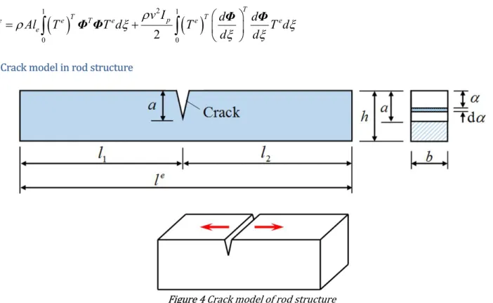
3.2 Crack model in rod structure
Figure 4 Crack model of rod structure
Due to the influence of axial force, the opening crack mainly occurs in the axial rod. The spring used to simulate the crack in rod only has axial stiffness, and the axial flexibility of spring
c
a can be calculated based on Castigliano'stheorem shown in Przemieniecki (1985) and Tada et al. (2000)
2 2 02
a ac
f
d
Eb h
(25) Where,
3 Ι0.752 2.02 /
0.37 1
/ 2
tan
/ 2
/ 2
/ 2
h
sin
h
h
f
h
cos
h
4. Numerical Examples
Several numerical examples of wave propagation simulation in rod structures are proposed to validate the Laplace based wavelet finite element method, a uniform rod is used in the numerical simulation, the geometry parameter and material properties are shown in Table 1.
Table 1: Geometry parameter and material properties of the rod structure
Length(mm) 1500
Young’s modulus(GPa) 200
Poisson’s ratio 0.3
Density(kg/m3) 7800
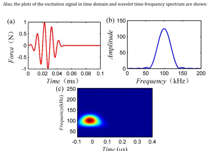
An excitation signal with 5-cycle sinusoidal tone burst is picked for wave propagation simulation in rod structure, the single central frequency of which is 100kHz, and the largest frequency is 150khz as shown in Fig. 5. The excitation signal in time domain is listed in Eq. 27.
1
2
1 cos 40
sin 200
0
0.05
0
t
ms
t
t
f t
others
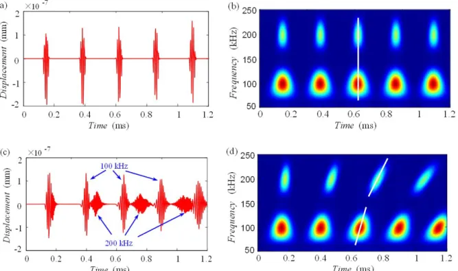
(27)Also, the plots of the excitation signal in time domain and wavelet time-frequency spectrum are shown in Fig. 5.
Figure 5: Excitation signal: (a) Time-domain diagram; (b) Frequency spectrum; (c) Wavelet time-frequency spectrum
Since the element size and time step increment are dependent on the wavelength of the excitation signal, which is related with the maximum frequency. The largest frequency of interest for this excitation signal is defined as
150
maxf
kHz
. Thus we could get the minimum period for this signal isT
min
6.67
s
with the shortestthe time interval is
t T
min/ 20 0.33
s
. Since the length of excitation signal ist
f
0.05
ms
, the sample pointsare set as
N t
f/
t
1
.4.1 Numerical simulation of ultrasonic wave propagation in rod with different methods
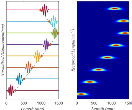
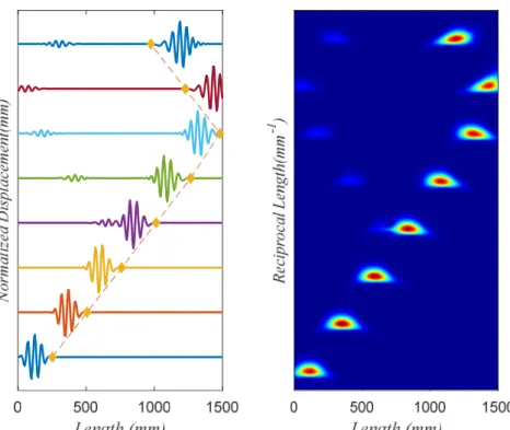
Firstly, a comparison of ultrasonic wave propagation in rod between Laplace based BSWI method and theoretical group velocity is compared in Fig. 6.
Figure 6. Left: Wave propagation comparison in rod between Laplace based BSWI method and theoretical group velocity; Right: Time frequency analysis results of the displacement signal at different time
As we could see from Fig. 6, the Laplace based BSWI method could provide very reliable results of ultrasonic wave propagation in rod. And we would like to study the advantages and disadvantages of this method. For comparison, conventional FEM would also be applied to compare the advantages and disadvantages between the two methods. From the time frequency analysis of the wave propagation in rod structure, the central frequency is moving along the rod as the wave propagate along the rod, which also proves the validity of our method.
Firstly, in order to study the influence of element size on the simulation results, different element size with same time intervals for these three methods are studied, the time interval is set as
t T
min/ 20 0.33
s
toensure 20 integration time steps per period, while the element size or the number of elements per wavelength (EPW) is different. The displacement response at the middle point of the rod is picked for comparison for these two different numerical methods. Also the EPW is different for different simulation methods. For conventional FEM, the EPW is set as 5, 10, 15, 20, the simulation result for conventional FEM with different EPWs is shown in Fig. 7. As can be seen from the plot, the arrival time for different wave packets could be got and the group velocity could be calculated and the value is 5053m/s when the EPW is 20, the calculated velocity is very close to the theoretical group velocity of aluminum rod is
c
0
E
/
5063 /
m s
. In comparison, in the Laplace based wavelet finiteFigure 7. Comparison between FEM and LWFEM for sensitivity study of element size
Another important factor in finite element method for time integration is the setup of time step, selecting a good value for time interval is so important that it could influence the accuracy of the results as well as the time cost during computation. So choose an appropriate time interval value which could both ensure the accuracy of results and not let the time cost be too high. Here we would like to come up with a concept of number of integration steps per period (denoted as SPP). For finite element method, we would like to set SPP as 10, 15, 20, 25, and the SPP is set as 1, 2, 4, 6. And the comparison results for the two methods are shown in Fig.8. As shown in Fig.8, the finite element method would converge quickly when SPP is larger than 15, but the same value for LWFEM is 2. From the comparison we could see that finite element method needs smaller time step, while the LWFEM would only need 1/5 of the time interval needed by finite element method.
Figure 8. Comparison between FEM and LWFEM for sensitivity study of time interval
4.2 The velocity dispersion in rod
Wavelet transform could provide more information on ultrasonic wave propagation in rod structure. Since wavelet transform is a very good time-frequency analysis tool, so we would like to study the time-frequency properties of ultrasonic wave propagation in rod structure. A new excitation signal is proposed to study the velocity dispersion of guided waves in rod structure, where double center frequencies 100Khz and 200Khz are included in this excitation signal. Also, the equation of this new excitation signal is shown in Eq.26 and the plots information shown in Fig.9:
1
2
1 cos 40
1
2
sin 200
1
2
400
0
0.05
0
t
t
sin
t
t
ms
f t
others
Figure 9 Excitation signal for velocity dispersion study: (a) Time-domain diagram; (b) Frequency spectrum; (c) Wavelet time-frequency spectrum
Both rod elements proposed in previous sections are applied to find the ultrasonic wave propagation response at the middle of the rod by LWFEM. Firstly, the wave propagation response and the velocity dispersion in classical rod structure and in Rayleigh-love rod are shown in Fig.10.
Figure 10 The displacement responses at middle point of rod subjected to excitation II: (a, b) Time-domain diagram and Wavelet time-frequency spectrum simulated by classic rod; (c, d) Time-domain diagram and Wavelet time-frequency
The classical BSWI rod element and the Rayleigh-Love BSWI rod element are respectively used to simulate the same rod which is divided into 48 BSWI rod elements. For classical rod theory, the velocity dispersion can’t be considered and the waveforms almost have no change in the process of propagation, as shown in
Figure 10 (a, b), because the waves of each frequency component propagate at the same rod speed. However, for the Rayleigh-Love rod theory, it is can be seen from Fig. 10 (c, d) that the two waveforms are gradually separated and the amplitudes of waveforms attenuate gradually in time history. The group velocities of waves in the vicinity of 100Hz change slowly, while those of in the vicinity of 200Hz have lower speeds and change more quickly. When the ratio of the cross-section size to the wavelength is less than 0.7, the Rayleigh-Love rod theory is able to give a good approximation for the dispersion proposed by Doyle (1997). Otherwise, it is necessary to develop and apply the complex multi-dimension theory.
Hence, the development and select of proper BSWI element is the critical for FFT-based BSWI method to simulate wave propagation. And it is an important preparation for SHM to select the proper frequency and mode of wave according to the dispersion property of waves.
4.3. Nondestructive testing in cracked rod structure with LWFEM
Figure 11. Left: Wave propagation in rod with crack in the middle of rod with Laplace based BSWI method; Right: Time frequency analysis of the wave signal in rod
Figure 11 shows the ultrasonic guided wave propagation in the rod with crack in middle of rod, in which the excitation signal is shown in Eq. 25 and the crack depth is 20% of the width of the rod. As we could see from this plot, the waveform at time
200
s
is different from the waveform at time150
s
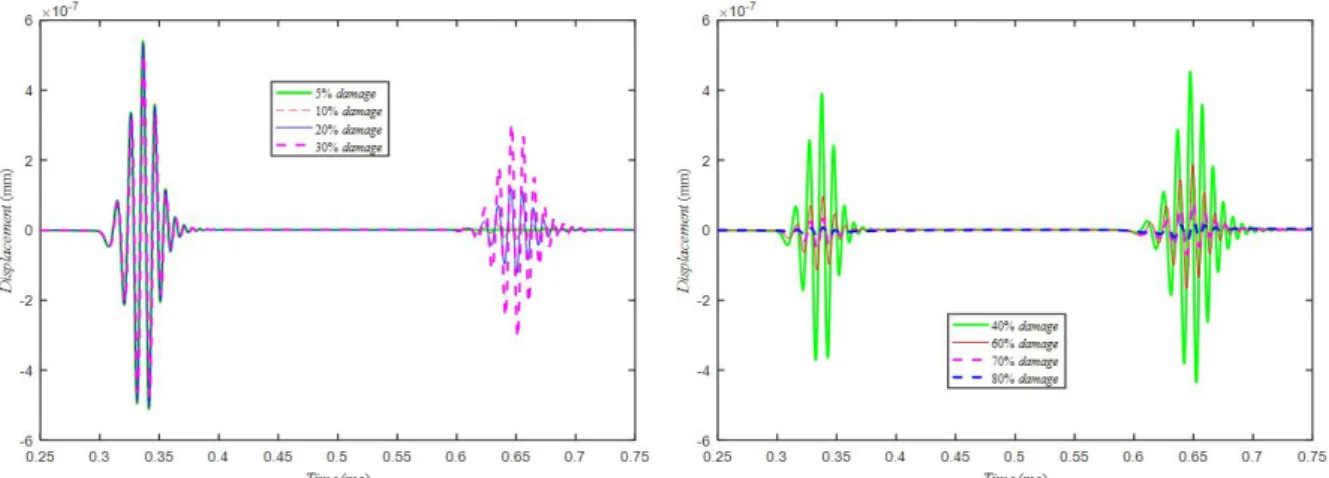
, which means that there is a wave that is reflected by the crack. Also as the time goes, the waveform reflected by the crack is more and more obvious, while the excitation wave would go across the crack and propagate along the rod structure until it is reflected by the right end of the rod again, at the same time, the wave reflected by the crack would propagate along the rod to the left end and is reflected by the left end of the rod. The time frequency analysis results of the wave propagation signal along the rod structure shows the central frequency is moving along the rod, and the central frequency is separated into two parts as the wave signal is passing the damage.Figure 12. Wave propagation in rod with crack in the middle of rod with different crack depth
The percentage of damage is evaluated as the ratio of crack depth with respect to the height of rod. As we could see from the left plot in Fig.12, the signal directly received by the right end of the rod structure is almost the same when the damage is small when the damage ratio is below 30%, but the amplitudes of the flaw signal received by the right end are highly influenced by crack depth. The amplitude of the flaw signal is proportional to the crack depth, the amplitude of the flaw signal would go up as the crack depth increases. Also the amplitude of direct wave signal would decrease when the crack depth increases if we take a look at the right plot of Fig.12. As shown in Fig. 12, the amplitude of both direct wave signal and flaw wave signal would decrease when the crack depth is increasing.
Another important factor that we studied in this manuscript is the crack location, which is shown in Fig. 13. In this case, we applied the same excitation signal on the left end and receive the signal on the right end of the rod, the depth of the cracks are set as 0.2h, while the locations are set different, one of the cracks is set in the middle of the rod while the other crack is set at the location of 1/4l. As we could see from Fig.14 that there are more flaw waves when the crack is located at the 1/4l with the same time length. Also the direct waves received by the right end of rod are the same.
Fig.13. Wave signal received by the right end of rod with different crack locations: Left-0.5l; Right-0.25l
Fig.14. Wave signal received by the right end of beam with multiple cracks
5. Conclusion
In this manuscript, a novel numerical Laplace based wavelet finite element method is proposed for ultrasonic wave propagation and nondestructive testing in rod structures. Laplace transform is a more advanced method than fast Fourier transform that Laplace transform does not depend on the periodic assumption while Fourier transform does. Also BSWI is a wavelet based finite element method that has been used in ultrasonic wave propagation and has a lot of advantages. By combining the advantages of the two methods, the following conclusions could be achieved:
1. Laplace transform is a symbol-based transform method, but still could be achieved via numerical method, but Laplace transform could abandon the periodic assumption of FFT.
2. By comparing the group velocity and wave propagation in rod, we could see that LWFEM is a very reliable numerical method that could be used in ultrasonic wave propagation and nondestructive testing of rod structures.
3. By studying the sensitivity of mesh size and time interval with different numerical methods, we could conclude that LWFEM has much lower element size and time interval requirement than traditional FEM but could still provide the necessary accuracy of results. Although it shows similar results with FFT based FEM, this is because both methods are solved in frequency domain and the two methods have similarities.
4. The velocity dispersion could not be clearly recognized and the waveforms almost have no change in the process of propagation in the classical rod element theory, while the Rayleigh-Love rod theory is able to give a good approximation for the dispersion when the ratio of the cross-section size to the wavelength is less than 0.7.
5. LWFEM is a reliable numerical method for nondestructive testing in rod structure and could recognize both small and large damages in the rod structure. Also the crack location also has a great influence on the received signals on the rod structure.
6. The signal directly received by the right end of the rod structure is almost the same when the damage is small when the damage ratio is below 30%, but the amplitude of direct wave signal would decrease when the crack depth increases. Also the amplitudes of the flaw signal received by the rod are highly influenced by crack depth, which was proved by FFT based BSWI simulation results. Multiple cracks problem in rod is studied with LWFEM, which shows that LWFEM could be successfully applied in complex nondestructive testing environments.
5. Acknowledgment
The authors are grateful for the financial support from National Natural Science Foundation of China (NSFC) under Grant No. 51478079, and the National Fundamental Research Program of China under Grant Nos. 2011CB013703, DUT15LAB11 and Natural Sciences Found of China (No. 51708251).
References
Chen, Y., Khandaker, M., & Wang, Z. (2017b, September). Secure in-cache execution. In International Symposium on Research in Attacks, Intrusions, and Defenses (pp. 381-402). Springer, Cham.
Chen, H., et al. (2007). “Vibration-based damage detection in composite wingbox structures by HHT.” Mechanical systems and signal processing 21(1): 307-321.
Chen, X., et al. (2012). “Modeling of wave propagation in one-dimension structures using B-spline wavelet on interval finite element.” Finite Elements in Analysis and Design 51: 1-9.
Chen, Y., Joffre, D., & Avitabile, P. (2018). Underwater Dynamic Response at Limited Points Expanded to Full-Field Strain Response. Journal of Vibration and Acoustics, 140(5), 051016.
Chen, Y., Zhang, B., Zhang, N., & Zheng, M. (2015). A condensation method for the dynamic analysis of vertical vehicle–track interaction considering vehicle flexibility. Journal of Vibration and Acoustics, 137(4), 041010.
Dai, N., et al. (1995). “Wave propagation in heterogeneous, porous media: a velocity-stress, finite-difference method.” Geophysics 60(2): 327-340.
Doyle, J. F. (1989). Wave propagation in structures. Springer: 126-156.
Doyle, J. F. (1997). Wave propagation in structures: spectral analysis using fast discrete Fourier transforms. New York, Springer.
Goswami, J. C., et al. (1995). “On solving first-kind integral equations using wavelets on a bounded interval.” IEEE Transactions on antennas and propagation 43(6): 614-622.
Harari, I. and E. Turkel (1995). “Accurate finite difference methods for time-harmonic wave propagation.” Journal of Computational Physics 119(2): 252-270.
Hu, Z. (2017). Contact Around a Sharp Corner with Small Scale Plasticity. Adv. Mater.,6, 10-17.
Hu, Z., Lu, W., Thouless, M.D., Barber, J.R., 2015. Simulation of wear evolution using fictitious eigenstrains. Tribology International 82, Part A, 191-194.
Hu, Z., Lu, W., Thouless, M.D., Barber, J.R., 2016. Effect of plastic deformation on the evolution of wear and local stress fields in fretting. International Journal of Solids and Structures 82, 1-8.
Hu, Z., Pratt, J.W., 2010. The Environmental and Economic Impact of IGCC in China, With Comparison to Alternative Options, Proceeding of ASME International Conference on Energy Sustainability, Volume 1, Phoenix, Arizona.
Igawa, H., et al. (1999). Wave propagation analysis of frame structures using the spectral element method. SPIE proceedings series, Society of Photo-Optical Instrumentation Engineers.
Kudela, P., et al. (2007). “Wave propagation modelling in 1D structures using spectral finite elements.” Journal of Sound and Vibration 300(1): 88-100.
Li, D., et al. (2014). “Corrosion monitoring and evaluation of reinforced concrete structures utilizing the ultrasonic guided wave technique.” International Journal of Distributed Sensor Networks 2014.
Liu, Z., Cheng, K., Li, H., Cao, G., Wu, D. and Shi, Y. (2018a). Exploring the potential relationship between indoor air quality and the concentration of airborne culturable fungi: a combined experimental and neural network modeling study. Environmental Science and Pollution Research, pp.1-8.
Liu, Z., Wu, D., Yu, H., Ma, W. and Jin, G. (2018b). Field measurement and numerical simulation of combined solar heating operation modes for domestic buildings based on the Qinghai–Tibetan plateau case. Energy and Buildings, 167, pp.312-321.
Ma, J., et al. (2003). “A study of the construction and application of a Daubechies wavelet-based beam element.” Finite Elements in Analysis and Design 39(10): 965-975.
Marfurt, K. J. (1984). “Accuracy of finite-difference and finite-element modeling of the scalar and elastic wave equations.” Geophysics 49(5): 533-549.
Mitra, M. and S. Gopalakrishnan (2005). “Spectrally formulated wavelet finite element for wave propagation and impact force identification in connected 1-D waveguides.” International Journal of Solids and Structures 42(16): 4695-4721.
Moser, F., et al. (1999). “Modeling elastic wave propagation in waveguides with the finite element method.” Ndt & E International 32(4): 225-234.
Park, J. (2015). “Lumped Parameter Model for a Self Powered Fontan Palliation of the Hypoplastic Left Heart Syndrome.”
Park, J. H., Nair, S., & Kim, D. (2017, April). Numerical analysis of helical dielectric elastomer actuator. In SPIE Smart Structures and Materials+ Nondestructive Evaluation and Health Monitoring (pp. 101631A-101631A). International Society for Optics and Photonics.
Przemieniecki, J. S. (1985). Theory of matrix structural analysis, Courier Corporation.
Rose, J. L. (2003). “Boundary element modeling for defect characterization potential in a wave guide.” International Journal of Solids and Structures 40(11): 2645-2658.
Royston, T.J., Dai, Z., Chaunsali, R., Liu, Y., Peng, Y. and Magin, R.L. (2011). Estimating material viscoelastic properties based on surface wave measurements: A comparison of techniques and modeling assumptions. The Journal of the Acoustical Society of America, 130(6), pp.4126-4138.
Saenger, E. H., et al. (2000). “Modeling the propagation of elastic waves using a modified finite-difference grid.” Wave motion 31(1): 77-92.
Seemann, W. (1996). “Transmission and reflection coefficients for longitudinal waves obtained by a combination of refined rod theory and FEM.” Journal of Sound and Vibration 198(5): 571-587.
Shen, W., et al. (2017). “Analysis of wave motion in one-dimensional structures through fast-Fourier-transform-based wavelet finite element method.” Journal of Sound and Vibration 400: 369-386.
Tada, H., et al. (2000). “The stress analysis of cracks handbook ASME.” New York: 55-56.
Tang, Q. and Yu, T. (2017). Finite element simulation of ultrasonic waves in corroded reinforced concrete for early-stage corrosion detection. In Nondestructive Characterization and Monitoring of Advanced Materials, Aerospace, and Civil Infrastructure 2017 (Vol. 10169, p. 101691N). International Society for Optics and Photonics.
Advanced Materials, Aerospace, Civil Infrastructure, and Transportation XII (Vol. 10599, p. 105991N). International Society for Optics and Photonics.
Xiang, J., et al. (2007). “The construction of 1D wavelet finite elements for structural analysis.” Computational Mechanics 40(2): 325-339.
Xiang, J., et al. (2013). “Detect damages in conical shells using curvature mode shape and wavelet finite element method.” International Journal of Mechanical Sciences 66: 83-93.
Yam, L., et al. (2003). “Vibration-based damage detection for composite structures using wavelet transform and neural network identification.” Composite Structures 60(4): 403-412.
Zhang, Z., Drapaca, C., Zhang, Z., Zhang, S., Sun, S., & Liu, H. (2017a). Leakage Evaluation by Virtual Entropy Generation (VEG) Method. Entropy,20(1), 14.
Zhang, Z., Ou, J., Li, D., & Zhang, S. (2017b). Optimization Design of Coupling Beam Metal Damper in Shear Wall Structures. Applied Sciences,7(2), 137.