Dynamics modelling of spot welded joints

Texto

(1)DYNAMIC MODELLING OF SPOT WELDED JOINTS Júlio M. M. Silva1, Fernando C. Batista2 and Nuno M. M. Maia1 1. Instituto Superior Técnico, Departamento de Engenharia Mecânica, Av. Rovisco Pais, 1096-001 Lisboa, Portugal 2 Escola Superior de Tecnologia e Gestão de Leiria, Departamento de Engenharia Mecânica, Morro do Lena, 2401-951 Leiria, Portugal e-mail: jms@alfa.ist.utl.pt. Abstract The determination of the dynamic characteristics of joints connecting structural components is a not yet solved problem of great importance when one intends to establish a theoretical model of the dynamic behaviour of a complex structure. Many of the problems found in such a process are in fact due to the difficulties related to the theoretical modelling of joints, be these connections of the classical type – welded, bolted, riveted, etc. - or still more complicated, as elastic supports, ribbons, etc. Given the complexity of the problem, it is convenient to approach it considering each specific type of joint separately. In the present case, the work will focus on spotwelded joints such as the ones found in the body of automobile vehicles. Spot-welds connect laminated foils, limiting to small areas the effective connecting zones. As a consequence, the application of common finite element techniques to the analysis of the dynamic behaviour of the vehicle body, yields not very accurate results given the fact that the effects of the welded connections are not accounted for. The objective of this work is to search for a simple numeric model that characterizes those joints, so that a more accurate model of this type of structures may be available..

(2) INTRODUCTION Purely theoretical analysis in dynamic studies is still somewhat unreliable in many situations. Experimental analysis is, therefore, needed in order to solve many real problems. A good example of this situation is the case of accounting for the influence of the joints in the dynamic behaviour of structures. This paper is intended to be a contribution for the search of simple solutions to the modelling of spot welded joints having in mind future applications to vehicle structures. Searching for the work of other researchers one can find a number of them interested in the same problem. A good recent example is found in Liu [1] who, in 2000, developed a model to describe the behaviour of a welding bead joining the tips of two beams. Vlahopoulos [2], in 1998, approached the finite element modelling of spot welds based on an energetic concept. Bearing in mind the particular case of vehicle structures and the development of computer codes for use in commercial programmes, CDH and BMW [3], in 1999, developed a model in MSC.NASTRAN called “linchweld”. Despite the fact that they claim that the model implies a substantial reduction in computer calculation time, little is known about this model. In the same year, MSC.NASTRAN presented a linear finite element called CWELD which was included in the module MSC.AMS-FVA of the UNIX version of the code [4]. This paper addresses the problem of taking into account the influence of spot welded joints in the dynamic behaviour of structural components through very simple modelling approaches. The study uses experimental modal analysis applied to two simple structural elements joined by spot welds. Results are presented and discussed.. BASIC CONSIDERATIONS The main concern for this study was to consider geometrically simple elements, easy to model using finite element techniques. This approach was followed so that the influence of the joining spot welds could be easily accounted for. Thus, the elements to be joined and analysed were chosen to be two rectangular steel plates. The study was also based on the following considerations: • • •. Model validation was based on the comparison of direct point frequency response functions obtained at the same point on all the structures under analysis; The comparison between theoretical and experimental results was made considering the first six natural frequencies of the structure; The frequency range of the analysis was 0-800 Hz for some of the plates and 0-400 Hz for the joined assemblies.. As said before, the structural elements used for this study were rectangular steel plates with small thickness, similar to the material used in vehicle bodies, so that spot welds could easily be used. Therefore, a thickness of 1,5 mm was chosen as adequate.

(3) to characterize that type of structures, like Wang [5] did, who also uses the same thickness in his work. Spot welding the plates implies superimposing the two elements (plates) to be joined. The superimposing width is normally around three times the welded zone diameter i.e., 18 mm. Five different coupling configurations were used in order to join the two plates, as shown in figure 1, with 1, 2, 3, 4 and 5 welded spots, always separated by the same distance of 50 mm (note that joined plates with the same geometric dimensions are denoted by the same letter). In order to avoid symmetry in the coupling configuration, two different types of plates were used: one with 300 mm length and the other with 400 mm length. The width of the plates varied from 100 mm to 250 mm according to the number of spot welds to be used. The main objective of avoiding symmetry was to avoid nodes of the vibration modes to occur on the welded joint, in order to make it easier to interpret the results. Also and in order to ensure validity of the results, tests were performed in six different sets of joined plates.. Figure 2 – Location of the response measuring accelerometer.. Figure 1 – The five different coupled elements.. PLATES MODELLING The main concern when modelling the plates was to guarantee that the finite element model would accurately simulate the plates individually. Thus, the discrepancies.

(4) found when analysing the joined assemblies could be, with certainty, due only to the influence of the joint. All the model characteristics (choice of finite element, model discretization, Young’s modulus, average size of the mesh and effect of additional mass due to the response measuring accelerometer) were carefully determined. The computer dynamic analysis code more commonly used in the automotive industry is MSC.Nastran. However, the authors could only use Ansys 6.0. [6] because this was the only code available.. Additional effect of the mass of the accelerometer As implied before, the experimental dynamic response of the structures under analysis was obtained through the use of an accelerometer. Thus, the mass of this measuring device (connected to the structure as shown in figure 2) was taken into consideration in the theoretical model. This procedure avoided any influence of the mass when comparing theoretical and experimental results. Also, the finite element mesh of all theoretical models included a node at the location where the geometrical centre of the accelerometer was attached ( Figure 3). Determination of the model characteristics The choice of the finite element to use, as well as the mesh size and the modulus of elasticity of the material, were considered as very important for an accurate modelling of the plates. For this purpose, a sensitivity analysis was carried out where the numerically obtained natural frequencies are compared with those obtained experimentally. In this case, the experimental response of the plates was determined using a non-contact laser vibrometer in order to avoid any extraneous influences in the results. Note that the laser vibrometer was not used in the subsequent measurements (an accelerometer was used as stated before) because its response was very noisy outside the natural frequency regions. Taking advantage of the finite element code library, a number of different structural elements was selected including both SHELL and SOLID elements. 5 mm 5 mm. Additional mass. Numerical model. Figure 3 – Location of additional mass on the numerical model.. After a number of analyses, the Young’s modulus was found as varying from 200GPa to 216 GPA. A mesh size varying from 6mm to 22 mm was also found to be.

(5) adequate. The relative error, as used by Lardeur [7], is defined between the experimental natural frequency obtained with the laser vibrometer and the theoretical natural frequency obtained with the finite element analysis. In this way, and assuming an error smaller than 0.5 %, the value of the Young’s modulus was taken as 213 GPa and the mesh size was chosen to be 10 mm using the finite element SHELL63.. EXPERIMENTAL ANALYSIS The experimental procedure was based on experimental modal analysis, simulating free-free conditions (to avoid border constraints that could influence the results) [8]. This was achieved suspending the plates, with nylon strings, from a structure so that the plates could oscillate in the direction of the vibration exciting force. For this purpose, two small holes were drilled in each plate. The experimental set-up included a spectral analyser OROS25 and a PC computer with data acquisition capabilities, as shown Figure 4. The excitation procedure was based on the impact technique using a hammer with a force transducer at the tip.. Figure 5 – Example of spot weld.. Figure 4 – Test set-up.. As far as the spot welds were concerned, care was taken in order to guarantee their precise location, marking carefully the plates as shown in figure 5. However and as can be seen in this same figure, this was extremely difficult to achieve and small offsets were always present.. RESULTS General observations In general it could be verified that the results obtained for the coupled assemblies with larger dimensions and hence, with more spot welds (assemblies type C and D – see figure 1), presented clearer discrepancies. In the case of assemblies type A and B, these discrepancies were only clearly observed for the higher natural frequencies. Tested models.

(6) Two different types of models are presented in this paper: i) One that considers the spot welds as connections where each of them joins a simple node on each plate (figure 6), and ii) one where the area limits of the welding spot are represented by various mesh nodes (figure 7) on each plate and the coupling procedure involves these nodes. Simple model This corresponds, in fact, to the model used by Wang [5] though this author used a beam to connect the two assembly elements. In our case, we started by just rigidly connecting the nodes that represent the centre of the spot weld on each plate.. Figure 6 – Simple model.. Figure 7 – Model with circle representing the outside limits of the spot weld.. The frequency response functions (FRFs) obtained for this model (red line) are presented in figure 8 where they are compared with the experimental results (blue line) for an assembly type A with a single spot weld joining the two plates. It is obvious from this figure that the rigid connection is not rigid enough as it does not accurately represent the stiffening effect of the spot weld. FRFs plates A1 (100mm) with 1 point. FRFs plates A1 (100mm) with 1 point 70. 70 Experim ental Rigid connection. 50. 50. 40. 40. 30. 30. 20 10 0 -10. mm mm mm mm mm mm. 20 10 0 -10. -20. -20. -30. -30. -40. -40 -50. -50 -60. Experim ental Beam 4 - Radius = 3 Beam 4 - Radius = 4 Beam 4 - Radius = 5 Beam 4 - Radius = 6 Beam 4 - Radius = 7 Beam 4 - Radius = 8. 60. Amplitude dB (ref. 1 m/s 2 N). 2. Amplitude dB (ref. 1 m/s N). 60. -60. 0. 25. 50. 75. 100. 125. 150. 175 200 225 Frequency [Hz]. 250. 275. 300. 325. 350. 375. 400. Figure 8 - FRF – Assembly type A with one spot weld – rigid connection of a single node. 0. 25. 50. 75. 100. 125. 150. 175 200 225 Frequency [Hz]. 250. 275. 300. 325. 350. 375. 400. Figure 9 - FRF – Assembly type A with one spot weld – connection modelled by a beam element BEAM4.

(7) An alternative to the previous approach is to follow Wang’s model [5], joining the two plates with a beam. The authors of this paper also tested this type of model, using a cylindrical beam element with with 12 dofs (6 at each beam tip). As expected, this model could not simulate the real assembly. In fact the increase in complexity brought nothing new if one compares it with the previously presented simple model. Actually, the beam introduced extra flexibility and thus, produced results further away from the experimental ones. Figure 9 shows the results comparing the experimental FRFs (wider blue line) with the theoretical predictions for connecting beams with different base radius. Complex model The results obtained with a model where the circular spot weld is represented by the node in the mesh coinciding with its centre clearly showed that this simple model can never simulate the real situation because, even considering a rigid connection, it does not impose the stiffening effect of the spot weld. Thus, it is necessary to account for the fact that the spot weld covers a small area of the plates and therefore, a more complex model was developed where the finite element mesh includes nodes on the circular outer limits of the area corresponding to the spot. Figure 10 shows the modified mesh with a circular zone representing the spot weld. The connecting points were represented by eight nodes on this circular region. In figure 11, the experimental results (wide blue line) are compared with the theoretical predictions, for different radius of the spot weld zone. It can be clearly seen, in figure 11, that increasing the radius of the circle one easily approaches the experimental results. Thus, it was concluded that this procedure could be used as a means of modelling spot welds. FRFs plates A1 (100mm) with 1 point 70 60 50 40. Amplitude dB (ref. 1 m/s 2N). 30 20 10 0 -10 -20 -30. Experim ental Radius = 3 m m Radius = 4 m m Radius = 5 m m Radius = 6 m m Radius = 7 m m Radius = 8 m m. -40. Figure 10- Mesh with nodes on the limits of the spot weld area.. -50 -60. 0. 25. 50. 75. 100. 125. 150. 175 200 225 Frequency [Hz]. 250. 275. 300. 325. 350. 375. 400. Figure 11 – Assembly type A with one spot weld – effect of the radius of the circular line where node connections are considered..

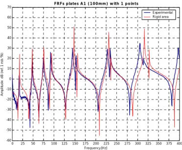
(8) However, the introduction of this circular zone, containing the connecting nodes, in the model mesh introduces a complexity that was originally meant to be avoided. In order to verify if the previous model could be simplified, a new model of the connections was implemented (figure 12) where the simulation of the joint was based on the nodes along the superimposed area of the plates. These nodes were rigidly connected and the results are presented in figure 13. The results in figure 13 show that this modelling procedure yields a stiffening effect that is greater than desired. After the second natural frequency, the stiffening effect is clearly seen. However, the results show that an approach such as this could be followed, playing with the mesh size and the number of connecting points. Thus, the simple mesh used to model the plates was considered again. The idea now is still to consider only the available nodes in this mesh. The spot weld joint was then represented by connections considering only the mesh nodes adjacent to the node representing the centre of the spot (figure 14). This time the authors searched for the more adequate mesh size, studying the assemblies with mesh sizes varying from 4.5 mm to 14 mm. FRFs plates A1 (100mm) with 1 points 70 Experim ental Rigid area. 60 50 40. Amplitude dB (ref. 1 m/s 2N). 30 20 10 0 -10 -20 -30 -40 -50 -60. 0. 25. 50. 75. 100. 125. 150. 175 200 225 Frequency [Hz]. 250. 275. 300. 325. 350. 375. 400. Figure 13 – Theoretical (red line) and experimental (blue line) results for assembly of plates type A using model of figure 12.. Figura 12- Model using the mesh nodes along the superimposed plates regions.. Figura 14- Model using rigid connections of nodes adjacent to the spot weld centre.. Also, the cases where the meshes of the two joined plates had no coincident nodes were analysed. It was found that good results could be obtained when the.

(9) meshes coincided (figure 15) whereas the non coincident meshes produced poorer results (figure 16). Figures 17 to 20 present results for different assemblies using mesh sizes of 4.5 mm and 9 mm. It may be concluded from these examples that the latter modelling approach is reasonably adequate in order to model the spot welds influence in the dynamic behaviour of the assembled structures. It must be noted that the results for the assemblies with only one spot weld are not so good mainly for higher frequencies. It is believed that this is due to the fact that, in this case, the model allows interpenetration of the two plates and thus, yields results that are not accurate. However, situations were only one spot weld exists are unrealistic. FRFs plates A1 (100mm) with 1 point. FRFs plates A1 (100mm) with 1 point. 70. 70 Experim ental Mes h= 4.5 m m Mes h= 9 m m. 50. 50. 40. 40. 30. 30. 20 10 0 -10. 20 10 0 -10. -20. -20. -30. -30. -40. -40. -50. -50. -60 0. 25. 50. 75. 100. 125. 150. 175 200 225 Frequency [Hz]. 250. 275. 300. 325. 350. 375. -60. 400. Figure 15 - FRF- Assembly type A with one spot weld –4.5 mm and 9 mm mesh Rigid connection of nodes adjacent to the spot. Coincident nodes.. 0. 50. 75. 100. 125. 150. 175 200 225 Frequency [Hz]. 250. 275. 300. 325. 350. 375. 400. FRFs plates B2 (150mm) with 3 points. FRFs plates A1 (100mm) with 2 point. 70 Experim ental Mes h= 4.5 m m Mes h= 9 m m. 60. Experim ental Mes h= 4.5 m m Mes h= 9 m m. 60 50. 40. 40. 30. 30 Amplitude dB (ref. 1 m/s 2N). 50. 20 10 0 -10. 20 10 0 -10. -20. -20. -30. -30. -40. -40. -50 -60. 25. Figure 16 - FRF- Assembly type A with one spot weld –6 mm and 8 mm mesh Rigid connection of nodes adjacent to the spot. Non coincident nodes.. 70. Amplitude dB (ref. 1 m/s 2N). Experim ental Mes h= 6 m m Mes h= 8 m m. 60. Amplitude dB (ref. 1 m/s 2N). Amplitude dB (ref. 1 m/s 2 N). 60. -50. 0. 25. 50. 75. 100. 125. 150. 175 200 225 Frequency [Hz]. 250. 275. 300. 325. 350. 375. 400. Figure 17 - FRF- Assembly type A with two spot welds – 4.5 mm and 9 mm mesh Rigid connection of nodes adjacent to the spot.. -60 0. 25. 50. 75. 100. 125. 150. 175 200 225 Frequency [Hz]. 250. 275. 300. 325. 350. 375. Figure 18 - FRF- Assembly type B with three spot welds – 4.5 mm and 9 mm mesh rigid connection of nodes adjacent to the spot.. 400.

(10) FRFs plates C 2 (200mm) with 4 points. FRFs plates D2 (250mm) with 5 points. 70. 70 Experim ental Mes h= 4.5 m m Mes h= 9 m m. 50. 50. 40. 40. 30. 30. 20 10 0 -10. 20 10 0 -10. -20. -20. -30. -30. -40. -40. -50 -60. Experim ental Mes h= 4.5 m m Mes h= 9 m m. 60. Amplitude dB (ref. 1 m/s 2N). Amplitude dB (ref. 1 m/s 2N). 60. -50. 0. 25. 50. 75. 100. 125. 150. 175 200 225 Frequency [Hz]. 250. 275. 300. 325. 350. 375. 400. Figure 19 - FRF- Assembly type C with four spot welds –4.5 mm and 9 mm mesh Rigid connection of nodes adjacent to the spot.. -60. 0. 25. 50. 75. 100. 125. 150. 175 200 225 Frequency [Hz]. 250. 275. 300. 325. 350. 375. 400. Figure 20 - FRF- Assembly type D with five spot welds –4.5 mm and 9 mm mesh Rigid connection of nodes adjacent to the spot.. CONCLUSIONS The problem of modelling structures with elements connected by spot welds was addressed. It was shown that simple models considering a single node to represent each connecting spot weld could not be used if accurate results were to be obtained. However, it was also shown that simple models can be used provided one considers the nodes adjacent to the spot weld centre as part of the modelled joint. REFERENCES [1]- Liu, Yanbin, Lim, C. Teik and Wang, Yi, Vibration Characteristics of Welded Beam and Plate Structures, Journal Noise Control Eng., 49(6), 2001. [2]- Vlahopoulos, N. and Zhao, X., An Approach for Evaluating Power Transfer Coefficients for Spot-Welded Joints in an Energy Finite Element Formulation, Journal [3]- Heiserer, D., Chargin, M., Sielaff, J., High Performance, Process Oriented, Weld Spot Approach, 1st MSC World Automotive, Munich, Germany, 1999 [4]- A. Jonscher, M. Lewerenz, G. Luehrs, The New Spot Weld Element in the CAE Process, Proc. of the 1st MSC World Automotive, Munich, Germany, 1999. [5]- Wang, Yi and Lim, C. Teik, An Experimental and Computational Study of the Dynamic Characteristics of Spot-Welded Sheet Metal Structures, SAE 2001 World Congress Detroit, 2001-01-0431, Michigan 2001. [6]- Ansys Manuals, version 6.0, 2001. [7]- Lardeur, P., Lacouture, E, Blain, E., Spot Weld Modelling Techniques and Performances of Finite Element Models for the Vibrational Behaviour of Automotives, Proc. of the 25th ISMA, Vol. 2, Leuven, Belgium, 2000. [8]- Maia, N. M. M., Silva, J. M. M. et al, Theoretical and Experimental Modal Analysis, Research Studies Press, UK, 1997.

(11)