A computable general equilibrium modeling platform for the azorean economy : a simple approach with international trade

(1)

WORKING PAPER SERIES

CEEAplA WP No. 09/2006

A Computable General Equilibrium Modeling

Platform for the Azorean Economy: A simple

approach with international trade

Ali Bayar Mário Fortuna Sual Sisik Cristina Mohora Francisco Silva July 2006

(2)

A Computable General Equilibrium Modeling

Platform for the Azorean Economy: A simple

approach with international trade

Ali Bayar

Universite Libre de Bruxelles

Departement D’Economie Appliquee

EcoMod

Mário Fortuna

Universidade dos Açores (DEG)

e CEEAplA

Sual Sisik

Universite Libre de Bruxelles

Departement D’Economie Appliquee

EcoMod

Cristina Mohora

Universite Libre de Bruxelles

Departement D’Economie Appliquee

EcoMod

Francisco Silva

Universidade dos Açores (DEG)

e CEEAplA

Working Paper n.º 09/2006

Julho de 2006

(3)

CEEAplA Working Paper n.º 09/2006 Julho de 2006

RESUMO/ABSTRACT

A Computable General Equilibrium Modeling Platform for the Azorean Economy: A simple approach with international trade

Computable general equilibrium models have become commonplace instruments of economic policy analysis in many developed countries. These models have gained increased acceptance due to their capacity to address many policy questions in a simple way, using now commonly available databases on the structure of production in the form of input-output matrices, while retaining traditional economic assumptions for household, firm and government behaviour, among others such as trade. In this paper we lay –out the model for application to the Azorean economy. The model contemplates households, firms, government, and trade. It is calibrated using a SAM built from a 1998 I-O table with all information updated to 2001. The impact of changes in trade is analysed.

Key words: CGE models; Ultra periphery; EU regional policy JEL classification: C68

Ali Bayar

Universite Libre de Bruxelles

Departement D’Economie Appliquee Avenue Paul Heger 2

B-1000 Bruxelles

Mário Fortuna

Departamento de Economia e Gestão Universidade dos Açores

Rua da Mãe de Deus, 58 9501-801 Ponta Delgada

Sual Sisik

(4)

Cristina Mohora

B-1000 Bruxelles

Francisco Silva

Departamento de Economia e Gestão Universidade dos Açores

Rua da Mãe de Deus, 58 9501-801 Ponta Delgada

(5)

A Computable General Equilibrium Modeling Platform for the Azorean Economy: A simple approach with international trade

Ali Bayar*, Mário Fortuna**, Sual Sisik*, Cristina Mohora*, Francisco Silva**

fortuna@notes.uac.pt

Abstract: Computable general equilibrium models have become commonplace

instruments of economic policy analysis in many developed countries. These models have gained increased acceptance due to their capacity to address many policy questions in a simple way, using now commonly available databases on the structure of production in the form of input-output matrices, while retaining traditional economic assumptions for household, firm and government behaviour, among others such as trade. In this paper we lay –out the model for application to the Azorean economy. The model contemplates households, firms, government, and trade. It is calibrated using a SAM built from a 1998 I-O table with all information updated to 2001. The impact of changes in trade is analysed.

Key words: CGE models; Ultra periphery; EU regional policy JEL classification: C68

Acknowledgments: This paper was written within the development of a project to

develop “An Instrument of Economic Policy Analysis for the Azores”, financed by several institutions, namely, the US Department of Agriculture, the Luso-American Development Foundation and the Regional Government of the Azores. The project was managed by CEEAplA, an FCT supported center of the Universities of the Azores and Madeira

(6)

1. Introduction

Analysing regional policy requires, quite often, that one look at the different levels of government that have a say in what exactly happens in one region. Depending on how government functions are set up, one might have to look at supra-national, national, regional and local government inputs into the policies that affect a certain region.

This is the case when we are analysing policy in the ultraperipheral regions of Europe. Even though French, Portuguese and Spanish regions are administered according to different political regimes, the set-up for policy analysis is the same. Some of the policies with significant impact in these regions are directly managed by the EU, some are managed by member state governments, others are the responsibility of the regional governments and yet some are managed by municipalities.

Construction of models capable of analysing not only ex-ante but also ex-post impacts of these policies is at a very incipient stage in all these regions. In the Azores and Madeira some econometric models have been specified to address very specific issues but with little use for current policy analysis (Fortuna, et al. (2006)). The same can be said for the other regions. Input-output models have been used in the past but not on a systematic basis.

Efforts are underway to surpass this gap with the construction of Computable General Equilibrium (CGE) models. CGE models have gained increased acceptance due to their capacity to deal with a wide variety of issues and to the fact that they do not require long statistical series as do econometric models (Menezes, et al (2006)). Even though constructing social accounting matrices is not as easy task, it is easier, in many cases, than obtaining relevant long series.

The purpose of the current paper is to specify the basic assumptions of a model to represent the economy of the Azores. This specification was made bearing in mind data limitations, at a first stage. The aim is to make the model increasingly more complex and capable of addressing ever more policy issues. The complexity of the model is constrained by data availability. The benefits of increased detail of policy analysis justify the effort put into data preparation.

In what follows we will start by describing the model, in detail, in section two. Section three briefly describes the data used and presents the model’s prediction of a variation in trade flows. Section four discusses the major shortfalls of the model and the recommended extensions. In the final section some concluding remarks are presented.

(7)

Model description

2.1. General outline of the model

The main objective of this project is to develop a multi-sectoral, multi-regional dynamic modeling platform of the Azores economy integrated within the European and global context. The platform will have the highest capabilities of analysis and forecasting in Azores for problems related to structural sectoral and regional issues, agriculture, labor markets, public finance, trade, EU funds, regional development, environment, and energy. The modeling platform is intended to act as an analytical and quantitative support for policy-making.

The first version of the modelling platform of the Azores economy is represented by a static multi-sectoral computable general equilibrium model (CGE), which incorporates the economic behaviour of four economic agents: firms, households, government and the rest of the world. All economic agents are assumed to adopt an optimizing behaviour under relevant budget constraints and all markets operate under the perfect competition assumption. The goods-producing sectors, consisting of both public and private enterprises, are disaggregated into 16 sectors1. The model distinguishes 16 types of commodities, such that each sector produces one homogenous commodity. With regard to the rest of the world the economy is treated as a small open economy with no influence on (given) world market prices.

Latter on, the core model for Azores will be developed into its multi-regional dimensions taking into account the islands or municipalities, depending on the data and needs. Dynamic feature will also be incorporated.

The core model for Azores is currently calibrated on the regional Social Accounting Matrix for 1998. The model has been solved by using the general algebraic modeling system GAMS (Brooke et al., 1998).

The following conventions are adopted for the presentation of the model. Variable names are given in capital letters; small letters denote parameters calibrated from the database (SAM) and elasticity parameters. Subscript sec stands for an identifier of one of the 16 production activities and one of the 16 commodities. Subscript ct stands for an identifier of the wholesale and retail trade services. Subscript nct stands for an identifier of one of the 15 commodities (except wholesale and retail trade services).

2.2. Firms

The CGE model does not take into account the behaviour of individual firms, but of groups of similar ones aggregated into sectors. The model distinguishes 16 perfectly competitive production sectors (summarized in annex I).

The usual assumption for such a model is that producers operate on perfectly competitive markets and maximize profits (or minimize costs) to determine optimal levels of inputs and output. For example, for the firms operating internationally, the world market dictates the output price to a large extent, so, for an optimal outcome they have to produce as efficiently as possible. Some other firms are constrained in the costs level by domestic competitors. Thus, the optimizing producers minimize their production costs at every output level, given their production technology. Furthermore, production prices equal average and marginal costs, a condition that implies profit maximization for constant returns to scale technology.

(8)

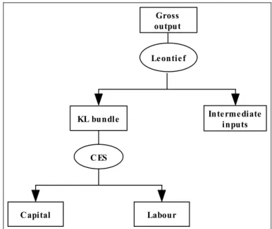
Gross output for each sector is determined from a nested production structure. At the outer nest producers are assumed to choose intermediate inputs and a capital-labour (KL) bundle, according to a Leontief production function, which assume an optimal allocation of inputs. At the second nest, producers choose the optimal level of labour and capital, according to a constant elasticity of substitution (CES) function which assumes substitution possibilities between labour and capital. Rigidities in the labour market are further introduced by the inter-sectoral wage differentials. The inter-sectoral wage differentials are derived as the ratio between the sectoral wage rate and the average wage rate at the national level (Dervis, De Melo and Robinson, 1982).

The demand equations for intermediate inputs, labour and capital and the corresponding zero profit conditions for these sectors are provided in annex II, equations (2.12.5)-(2.12.9). The nested structure and the functional forms used by these sectors are further given in figure 1.

Gross output KL bundle Leontief CES Labour Capital Intermediate inputs

Figure 1. The nested Leontief and CES production technology for the production sectors

Treated at an aggregate level, firms receive income from sales of goods; they purchase intermediate inputs, make wage payments and save (see equation(2.12.10), annex II).

2.3. Households

The households receive income from labour and a fixed share of the capital income and transfers from the government as unemployment benefits (see equation (2.12.2), annex II) and pay taxes on income to government and save a fixed fraction of net (money) income (see equation (2.12.3), annex II). Further, households’ budget devoted to consumption of commodities is given by the total income minus the taxes and savings (see equation(2.12.4), annex II). A schematic representation of households’ decisions is given in figure 2.

The optimal allocation between the consumption commodities ( C_sec) is given by

maximizing a Stone-Geary utility function: Hsec

U( C_sec) ( C_sec H_sec) sec

α µ

= ∏ − (1)

(9)

CBUD=(1-tsc_sec) (1+tc⋅ _sec)⋅P_sec⋅C_sec (2) where: _sec sec H 1 α = ∑ . sec

C represents the consumption of commodity sec by the households, P_sec is the consumer

price net of taxes for the commodity sec, µ_sec is the minimum (subsistence) level of consumption of commodity sec by the households, and αH_sec is the income elasticity of the

demand for commodity sec.

Sixteenth categories of consumer goods are distinguished. As already explained, each production sector is assumed to produce one homogenous commodity. Thus, the classification of the commodities follows the classification of the production sectors.

C apital supply Labor supply

Income from capital Labor de mand Une mployme nt Income from labor Une mployme nt be ne fits Income Taxe s on income House hold savings C ommoditie s (16 type s) C onsumption budge t

Figure 2. Decision structure of the households

Consumption is valued at consumer prices(1-tsc_sec) (1+tc⋅ _sec)⋅P_sec, which incorporate taxes on consumption (tc_sec) and subsidies on consumption( tsc_sec).

After some rearrangements, the optimization process generates the demand equations for consumption commodities (see equations(2.12.1), annex II)2.

To evaluate the overall change in consumer welfare we use the equivalent variation in income( EV ), which is based on the concept of a money metric indirect utility function

(Varian, 1992):

2_{The Linear Expenditure System (LES) was developed by Stone (1954) and represents a set of consumer demand}

(10)

sec

H

sec sec sec

sec sec PZ ( 1 tc0 ) ( 1 tsc0 ) EV = (V-VZ) H α α  ⋅ + ⋅ −  ⋅ ∏     (3)

The indirect utility function of the LES function in the counter-factual (policy scenario) equilibrium (V ) is defined as:

[

]

sec

sec sec sec sec

sec

H

sec V = CBUD- P ( 1 tc ) ( 1 tsc ) H H /(P ( 1 tc ) ( 1 tsc ))α µ α   ⋅ + ⋅ − ⋅ ⋅ ∑     ⋅ + ⋅ − ∏ (4)

and the indirect utility function of the LES function in the benchmark equilibrium (VZ )

is given by:

[

]

sec

H

sec VZ = CBUDZ- PZ ( 1 tc0 ) ( 1 tsc0 ) H H /(PZ ( 1 tc0 ) ( 1 tsc0 ))α µ α   ⋅ + ⋅ − ⋅ ⋅ ∑     ⋅ + ⋅ − ∏ (5)

whereCBUDZ reflects the household’s budget available for consumption in the

benchmark equilibrium,PZ_sec is the price of commodity sec in the benchmark and sec

tc0 and tsc0_sec are the consumption tax rate and the subsidy rate in the benchmark

equilibrium, respectively.

Equivalent variation measures the income needed to make the household as well off as she is in the new counter-factual equilibrium (policy scenario) evaluated at benchmark prices. Thus, the equivalent variation is positive for welfare gains from the policy scenario and negative for losses (Harrison and Kriström, 1997).

2.4. Government

Government revenues (TAXR) consist of taxes on households’ income, consumption taxes, taxes on investment goods and taxes on production plus transfers received by the government from the rest of the world:

sec sec sec sec sec sec sec sec

sec sec sec sec TAXR = ty YH + (P C (1-tsc ) tc +XD PD tp )+ P I tcinv +ER TRGW ⋅ ⋅ ⋅ ⋅ ⋅ ⋅ ⋅ ⋅ ⋅

∑

(6)

where ty is the tax rate on households income (YH ), tp_sec is the tax on production of sector

sec and tcinv_sec is the tax rate on investment good sec. XD_sec represents the gross output of

sector sec, where its price is given by PD_sec, and I_sec reflects the demand for the investment

commodity sec. The transfers received by the government from the rest of the world (TRGW)

are transformed in domestic currency by multiplying them with the exchange rate (ER).

Government expenditures (GEXP) consists of disposable budget for current consumption (CGBUD), unemployment benefits to the households’ and subsidies on consumption and production:

sec sec sec sec sec sec sec

(11)

where UNEMP represents the number of unemployed, PL is the average wage rate, trep is

the replacement rate out of the average wage rate, tsc_sec is the subsidy rate on consumption

of commodity sec and tsp_sec is the subsidy rate on production of sector sec.

Thus, government savings are given by the difference between government revenues and government expenditures:

SG = TAXR-GEXP (8)

The optimal consumption of commodities by the government is given by the maximization of a Cobb-Douglas utility function:

sec sec CG U( CG ) _CGsec sec α = ∏ (9)

subject to the budget constraint: sec sec sec CGBUD =

∑

CG ⋅P (10) with: _sec sec CG 1 α =

∑ . The optimization process yields the demand equations for each type of commodity (see equation (2.12.13), annex II).

2.5. Foreign trade

The specification of foreign trade is based on the small-country assumption, which means that the country is a price taker in both its imports and exports markets. As a result, both world import prices and world export prices are exogenously fixed. Two main groups of trading partners are distinguished in the model: the Mainland and the rest of the world.

The assumption of limited substitution possibilities between domestically produced and imported goods, which goes back to Armington (1969), is now a standard feature of applied models and will also be adopted here. It indicates that domestic consumers use composite goods ( X_sec) of imported and domestically produced goods, according to a CES function:

sec sec

A A

sec sec sec sec sec sec

A 1 A sec sec X aA ( A1 MML A2 MROW A3 XDD ) ρ ρ ρ ρ γ γ γ − − − − = ⋅ ⋅ + ⋅ + ⋅ (11)

Minimizing the cost function:

Cost ( MML ,MROW , XDD ) PMML MML

PMROW MROW PDD XDD

= ⋅ +

⋅ + ⋅ (12)

subject to (11), yields the demand equations for imports from Mainland ( MML_sec), for

imports from the rest of the world ( MROW_sec) and domestically produced goods sec

( XDD ) (see equations (2.12.16)-(2.12.18), annex II); where aA_sec is the efficiency

parameter, γA1_sec, γA2_sec, γA3_sec are the distribution parameters and the elasticity of

substitution between imports from different regions and domestically produced goods sec

( Aσ ) is given by 1 ( 1+ρA_sec). PMML_sec is the domestic price of imports of

commodity sec from Mainland including trade margins, PMROWsec is the domestic price of imports of commodity sec from the rest of the world including trade margins,

(12)

and PDD_sec is the price of domestically produced commodity sec delivered to the

domestic market also including trade margins.

The corresponding zero profit condition for the CES function is given by:

P ⋅X = PMML ⋅MML + PMROW ⋅MROW +PDD ⋅XDD (13)

where Psec is the composite price of commodity sec net of taxes.

A limited substitution is also assumed to exist between goods produced for the domestic market ( XDD_sec), exports to Mainland ( EML_sec) and exports to the rest of the world

sec

( EROW ), as captured by a constant elasticity of transformation (CET) function:

sec sec

T T

T 1 T sec sec XD aT ( T1 EML T 2 EROW T 3 XDD ) ρ ρ ρ ρ γ γ γ − − − − = ⋅ ⋅ + ⋅ + ⋅ (14)

where aT_sec is the efficiency parameter, γT1_sec, γT 2_sec, γT 3_sec are the distribution parameters, and the elasticity of substitution ( Tσ _sec) between exports to different

regions and domestically produced goods delivered to domestic market is given by sec

1 ( 1+ρT ).

By maximizing the revenue function of the producer:

Re venue ( EML ,EROW , XDD ) PEML EML

PEROW EROW PDS XDD

= ⋅ +

⋅ + ⋅ (15)

subject to (14) we derive the demand equations for exports and domestically produced goods (see equations (2.12.20)-(2.12.22), annex II), where PEML_sec is the domestic

price of exports of sector sec to the Mainland, PEROW_sec is the domestic price of exports of sector sec to the rest of the world, and PDS_sec is the price of domestic output

of sector sec delivered to domestic market excluding trade margins. The zero profit condition for the CET function is further given by:

PD ⋅XD = PEML ⋅EML +PEROW ⋅EROW + PDS ⋅XDD (16)

where PD_sec is the price of output produced by sector sec. Both exports and domestic

output delivered to the domestic market are valued at basic prices, PEML_sec, PEROW_sec

and PDS_sec.

The balance of payments is now determined as all international incoming and outgoing payments have been taken into account:

sec

(MML PWMMLZ +MROW PWMROWZ ) =

( EML PWEMLZ +EROW PWEROWZ ) TRGW+SW+LW PLWZ

⋅ ⋅

∑

⋅ ⋅ + ⋅

∑

(17)

The surplus/deficit of the balance of payments ( SW ), expressed in foreign currency, is

determined by the difference between imports and exports, valued at world prices, the transfers received by the government from the rest of the world (TRGW) and the labor

income from non-residential firms (LW PLWZ)⋅ , where PWMMLZsecis the foreign price of imports of commodity sec from the Mainland, PWMROWZ_sec is the foreign price of

(13)

the foreign prices of exports of sector sec to the Mainland and to the rest of the world, respectively.

2.6. Investment demand

Total national savings are given by: sec sec

S = SH + SF + SG - SW ER +⋅ ∑ DEP ⋅PI (18)

where SH are the households’ savings, SF firms savings, SG government savings and

sec

DEP is the depreciation of the capital stock. Depreciation is modelled as a fixed share of

capital stock (see equation (2.12.26), annex II).

The demand for investment commodities by type of commodity ( I_sec) is modelled in a

simple way, by maximizing a Cobb-Douglas utility function:

sec

I

sec sec

sec

U( I )= ∏Iα (19)

subject to the budget constraint:

sec sec sec sec sec

sec sec

S−

∑

SV ⋅P =

∑

I ⋅P ⋅ +( 1 tcinv ) (20)

with _sec secαI 1

=

∑ , where SV_{s ec} are the changes in stocks of commodity sec and tcinv_sec is

the tax rate on investment commodity sec. Changes in stocks are modelled in this case as a fixed share out of supply of commodities (see equation (2.12.27), annex II). Further, the maximization process yields the demand equations for investment commodities by type of commodity (see equation (2.12.28), annex II). The price of the composite investment commodity is further given by:

sec

I

sec sec sec

sec

PI = ∏[(P ⋅(1+tcinv ) ) / Iα ]α (21)

2.7. Price equations

A common assumption for CGE models, which has also been adopted here, is that the economy is initially in equilibrium with the quantities normalized in such a way that prices of commodities equal unity. Due to the homogeneity of degree zero in prices, the model only determines relative prices. Therefore, a particular price is selected to provide the numeraire price level against which all relative prices in the model will be measured. In this case, the GDP deflator (GDPDEF) is chosen as the numeraire.

Different prices are distinguished for all producing sectors, exports and imports. The domestic price of exports to Mainland ( PEML_sec) reflects the price received by the

domestic producers for selling their output to the Mainland, where PWEMLZ_sec is the

foreign price of exports to Mainland and ER is the exchange rate. The cost of trade

inputs further reduces the domestic price received by the producers:

sec sec ct,sec ct

ct

PEML =PWEMLZ ⋅ER−

∑

tcoeml ⋅P (22)

where tcoeml_{ct ,sec} is the quantity of commodity ct as trade input per unit of commodity

(14)

wholesale and retail sale commodity. In a similar way is defined the domestic price of exports to the rest of the world (see equation (2.12.38), annex II).

The domestic price of imports from Mainland ( PMML_sec) is determined by the foreign

price of imports from Mainland ( PWMMLZ_sec), the exchange rate, and the cost of trade inputs for imports:

ct

PMML = ER PWMMLZ⋅ + tcomml

∑

⋅P (23)

where tcomml_ct,sec is the quantity of commodity ct as trade input per imported unit of commodity sec.

The model distinguishes the price of domestic output supplied to domestic market paid by the consumers (PDD_i) and the price received by the producers (PDS_i). The difference

between the two prices is represented by the cost of trade inputs for domestic output delivered to domestic market:

sec sec ct,sec ct ct

PDD =PDS +

∑

tcod ⋅P (24)

where tcod_ct,sec is the quantity of commodity ct as trade input per unit of commodity sec delivered to the domestic market.

The consumer price index (INDEX) used in the model is of the Laspeyres type and is

defined as:

sec sec sec sec sec

sec INDEX = P CZ (1+tc ) (1-tsc ) / PZ CZ (1+tc0 ) (1-tsc0 ) ⋅ ⋅ ⋅     ⋅ ⋅ ⋅    

∑

(25)

Furthermore, GDP deflator is defined as the ratio of GDP at current market prices to GDP at constant prices (see equation (2.12.42), annex II).

2.8. Labour market

Labour services are used by firms in the production process (see equation (2.12.7), annex II). The model also allows for endogenous unemployment. Thus, the average wage rate paid by the firms is a function of consumer prices and the unemployment rate, as follows:

(

)

( ) /( ) 1

PL INDEX PLZ INDEXZ

beta UNEMP LSR UNEMPZ LSRZ

− =

⋅ − (26)

where LSR is the domestic labor supply, PL is the average wage rate in the current year and

beta is a parameter. PLZ , INDEXZ, UNEMPZ and LSRZ represent the average wage rate,

the consumer price index, the unemployment level and the domestic labor supply in the base year, respectively.

A labor supply curve, which assumes a positive correlation between the domestic labor supply and the real average wage rate:

elasLS

LSR = LSRZ ((PL INDEXZ)/(PLZ INDEX))⋅ ⋅ ⋅ (27)

is used to endogenize labor supply in the model, where elasLS is the real wage elasticity of labor supply.

(15)

Labour market is closed by changes in unemployment: sec sec LSK = LSR - UNEMP

∑

(28) where LSK_sec is the labor demand by sector sec. Further, total labor supply (LS) is given by:

LS=LSR LW+ (29)

where LW is the labor supply to non-residential firms.

2.9. Market clearing equations

Equilibrium in the product, capital and labour markets requires that demand equals supply at the prevailing prices (taking into account unemployment for the labour market). The clearing equation for the labour market has already been presented above (see equation (28)).

Similarly, the sum of demand for intermediate inputs nct (excluding the wholesale and retail trade commodity) of sector sec ( io_nct,sec⋅XD_sec), of demand for government and households consumption, of demand for investment goods and inventories must equal the supply of the composite good nct from domestic deliveries and imports (X_nct):

nct,sec sec nct nct nct nct nct sec

io ⋅XD +C +I +SV +CG = X

∑ (30)

For the wholesale and retail trade commodity the market clearing equation is given by:

ct,sec sec ct ct ct ct ct ct

sec

io ⋅XD +C +I +SV +CG +MARG = X

∑

(31)

where MARG_ct is the demand for trade services (Löfgren, Harris and Robinson, 2002). Total demand for trade services is further given by the sum of demand for trade services generated by the domestic output delivered to the domestic market, of the demand for trade services generated by the imports, and of the demand for trade services generated by the exports:

ct ct,sec sec ct,sec sec

sec

ct,sec sec ct,sec sec ct,sec sec

MARG = (tcod XDD +tcomml MML +

tcomrow MROW +tcoeml EML +tcoerow EROW )

⋅ ⋅

⋅ ⋅ ⋅

∑

(32) Further, capital stock is fixed by sector; therefore the equation for the clearing of the capital market has been dropped.

2.10. Closure rules

The closure rule refers to the manner in which demand and supply of commodities, the macroeconomic identities and the factor markets are equilibrated ex-post. Due to the complexity of the model, a combination of closure rules is needed. The particular set of closure rules should also be consistent, to the largest extent possible, with the institutional structure of the economy and with the purpose of the model.

To balance the number of endogenous variables and the number of independent equations in the model, additional assumptions are needed. Therefore, the transfers received by the government form the rest of the world and the labour income from non-residential firms is exogenously fixed in real terms. Further, in order to achieve the clearing of the labour market, inter-sectoral mobility of labour is assumed. However, the

(16)

presence of unemployment introduces rigidities in the labour market. The unemployment is endogenously determined through a wage curve. Labour supply is endogenously determined through a labor supply curve. On the capital market the sectoral capital stock is exogenously fixed, introducing rigidities.

The most widely accepted macro closure rule for CGE models implies the assumption that investment and savings balance. In the model, the investment is assumed to adjust to the available domestic and foreign savings. This reflects an economy in which savings form a binding constraint. The interest rate is assumed to effectively balance the supply and demand for investments, even if the specific mechanism is not incorporated in the model. This macro closure rule is neoclassical in spirit. However, the fact that the model allows for unemployment introduces a Keynesian element. As already mentioned, in models of this size it is not uncommon that a few closure rules are combined to get as close as possible to a realistic representation of the economy.

The government behaviour is modelled through an optimization process, which yields the optimal allocation of governments’ consumption by type of commodity. The budget deficits/surpluses of the government is fixed as a share of GDP. For the external sector, the surplus/deficit of the balance of payments is fixed and the endogenous exchange rate brings the balance of payments into equilibrium.

Gross domestic product is given at both constant prices and at current market prices (see equations (2.12.43)-(2.12.44), annex II). According to Walras’ law if (n-1) markets are cleared the nth one is cleared as well. Therefore, in order to avoid over-determination of the model, balance of payments equation (equation (17)) has been dropped. However, the system of equations guarantees, through Walras’ law, that its balance is equal to the difference between the exports and imports and the transfers from the rest of the world.

3. Data and Results

In order to calibrate the model data was collected to complete a SAM matrix. As referred before a 1998 input- output matrix for the Azores (Alves (2004)) was used. The sector detail was determined by the size of the input-output table, restricted to sixteen sectors. As a consequence, it is assumed that there are sixteen sectors all following the same optimizing behaviour. One single level of government was assumed. It was also assumed that there was a single household. Trade is done with two regions, the mainland and the rest of the world.

The structure of the economy was assumed not to change between 1998 and 2001. As such, all data, aside from the input-output table, was compiled for 2001.

On the basis of these assumptions the model was calibrated and a scenario was created to analyse the impact of a 10 % decrease in exports to the rest of the world.

Macroeconomic variables

GDP (% change) -0,22

Unemployment rate (%) 2,97

(17)

Welfare gains/losses (thousands EURO) -8.589 Welfare gains/losses (% of households income) -0,65

4. Model Extensions

The model presented above represents a first attempt at a comprehensive multi-sector modelling of the Azorean economy.

As it is specified, however, it does not contemplate a number of interesting policy issues. The following is a list of some of them:

a. not all sectors are competitive, transportation, energy supply and telecommunications being some of the most representative examples; b. all government expenditure is done through a single level of

government while in fact there are at least three relevant levels, the EU, the central and the regional;

c. trade occurs only with two regions, the mainland and the rest of the world, erasing some interesting regional ties such as the EU and the USA;

d. the sectors are too aggregated making it impossible to address sector specific issues such as dairy support policies or air transport support policies, for example;

e. there is a single household, which makes it impossible to analyse the redistributive impact of policies.

Depending on the objectives of analysis, other issues can also be added to the list. These are however those we consider more relevant and easily addressed. As such, work is underway to:

i. extend the detail of the SAM matrix to 45 sectors based on an input-output matrix constructed for 2001;

ii. extend the number of government agents to 4 – Foreign, EU, national, regional and municipal;

iii. make some of the sectors non-competitive;

iv. expand trade treatment to consider additional regions – mainland, EU, USA and rest of the world;

v. expand the number of households to three – low income, middle income and high income.

Other policy issues need also to be addressed such as trade restrictions and differentiated tax treatments.

5. Conclusion

In the above section we specified a simple CGE model with general characteristics of models of this nature. The purpose of the exercise was to arrive at a characterization of

(18)

the economy of the Azores, with a final objective of arriving at an instrument useful for economic and social policy analysis.

The model is standard in most respects but it was possible to use it in various exercises of the impact of policy measures and of external shocks. In one of the exercises conducted increased government expenditures were assumed. In another an external decrease in export demand was analysed. In both cases general impacts and detailed sector impact can be extracted from the output of the model.

The model, as specified, however, falls short of answering a series of interesting policy issues and is built on a data set that needs considerable improvement. The major shortfalls are associated to the lack of sector detail, desirable for analysing EU policies, for example, the concentration of government policy in one single level, lack of desegregation of trade partners, etc. These drawbacks set an agenda for new improvements in the model.

The current exercise, however, has constituted a positive contribution towards better characterizing the economy of the Azores and the impact of policies that, so far were only evaluated on the basis of empirical feelings and qualitative measures.

(19)

References

Armington, P. (1969). A theory of demand for products distinguished by place of production. IMFStaff Papers, 16, 159-178.

Brooke, A., Kendrick, D., Meeraus, A., & Raman, R. (1998). GAMS – A user’s guide. Washington: GAMS Development Corporation.

Alves, Brandão, e tal. (2004). Sistema de Matrizes Regionais Input-Output para a Região Autónoma dos Açores - 1998 . Presidência do Governo Regional dos Açores. Fortuna, M. Silva, F., Vieira, C., Dentinho, T. (2006). Modelling the Azorean Economy for Policy Analysis: a literature review. CEEAplA, working paper nº… University of the Azores.

Harrison, G. W., & Kriström B. (1997). General equilibrium effects of increasing carbon taxes in Sweden. Retrived from: http://www.sekon.slu.se/~bkr/Beijer.pdf. Löfgren, H., Harris, R. L., & Robinson S. (2002). A standard computable general equilibrium (CGE) in GAMS. IFPRI, Microcomputers in Policy Research, vol.5. Menezes, A., Fortuna, M., Silva, F., Vieira, J. (2006). Computable General Equilibrium Models: a literature review. CEEAplA, working paper nº… University of the Azores. Stone, R. (1954). Linear expenditure systems and demand analysis: An application to thepattern of British demand. Economic Journal, 64, 511-527.

Varian, H.R. (1992). Microeconomic analysis. New York: W.W. Norton.

Dervis, K., De Melo, J., & Robinson, S. (1982). General equilibrium models for

(20)

Annex I

Classification of the production sectors in the SAM and in the core model for Azores Table 17. Classification of the production sectors in the SAM and in the core model for Azores

Code Azores core model

Classification of the production sectors in the SAM and in AzoresMod NACE Division

sec1 Products of agriculture, hunting and forestry A

sec2 Fish B

sec3 Products from mining and quarrying C

sec4 Manufactured products D

sec5 Electrical energy, gas, steam and hot water E

sec6 Contruction work F

sec7

Wholesale and retail trade services; repair services of motor vehicles,

motorcycles and personal and household goods G sec8 Hotel and restaurant services H sec9 Transport, storage and communication services I sec10 Financial intermediation services J sec11 Real estate, renting and business services K

sec12

Public administration and defence services, compulsory social security

services L

sec13 Education services M

sec14 Health and social services N sec15 Other community, social and personal services O sec16 Private household with employed persons P

(21)

Annex II

Equations of the simulation model

2.11. Model equations 2.12.1. Households

sec sec c sec c sec c sec c

sec c P C ( 1 tc ) ( 1 tsc ) P H ( 1 tc ) ( 1 tc ) H ( CBUD H P ( 1 tc ) ( 1 tsc ) ) µ α µ ⋅ ⋅ + ⋅ − = ⋅ ⋅ + ⋅ − + ⋅ −

∑

⋅ ⋅ + ⋅ − (2.12.33)

sec sec YH = aich KSK RK LSK wdif PL trep PL UNEMP+PLWZ ER LW ⋅ ⋅ + ⋅ ⋅ + ⋅ ⋅ ⋅ ⋅

∑

(2.12.34) ( ) SH =mps YH ty YH⋅ − ⋅ (2.12.35)

CBUD = YH-ty YH-SH ⋅ (2.12.36)

2.12.2. Firms

sec sec sec

aKL ⋅XD = KL

(2.12.37)

sec sec sec sec sec sec secc,sec sec secc secc (1-tp +tsp ) PD⋅ ⋅XD = KL ⋅PKL +

∑

io ⋅XD ⋅P (2.12.38) sec sec sec P ( P -1) P

sec sec sec sec sec sec

LSK = KL ⋅[ PKL /(PL wdif⋅ )]σ ⋅γP2σ ⋅aPσ

(2.12.39)

sec sec sec P ( P -1) P

KSK = KL ⋅(PKL /(RK +d ⋅PI))σ ⋅γP1σ ⋅aPσ

(2.12.40)

PKL ⋅KL = RK ⋅KSK +DEP ⋅PI+PL LSK⋅ ⋅wdif

(2.12.41)

sec sec sec

SF = aicf⋅

∑

KSK ⋅RK

(22)

2.12.3. Government

sec sec sec

TAXR = ty YH + [P C (1-tsc ) tc +XD PD tp + P I tcinv ]+ER TRGW ⋅ ⋅ ⋅ ⋅ ⋅ ⋅ ⋅ ⋅ ⋅

∑

(2.12.43)

GEXP = CGBUD+trep PL UNEMP+⋅ ⋅

∑

[P ⋅C ⋅tsc +XD ⋅PD ⋅tsp ]

(2.12.44)

sec sec sec

P ⋅CG = Gα ⋅CGBUD (2.12.45) SG = TAXR-GEXP (2.12.46) RATIO = SG/GDPC (2.12.47) 2.12.4. Foreign trade sec sec sec

A (1 - A ) A

A (1 - A ) A (1 - A ) A /(1 - A )

MML = (X /aA ) ( A1 /PMML ) [ A1 PMML + A2 PMROW + A3 PDD ] σ σ σ σ σ σ σ σ σ γ γ γ γ ⋅ ⋅ ⋅ ⋅ ⋅ (2.12.48) sec sec sec

A (1 - A ) A

sec sec sec sec sec sec sec

A (1 - A ) A (1 - A ) A /(1 - A )

MROW = (X /aA ) ( A2 /PMROW ) [ A1 PMML +

A2 PMROW + A3 PDD ] σ σ σ σ σ σ σ σ σ γ γ γ γ ⋅ ⋅ ⋅ ⋅ ⋅ (2.12.49) sec sec sec

A (1 - A ) A

A (1 - A ) A (1 - A ) A /(1 - A )

XDD = (X /aA ) ( A3 /PDD ) [ A1 PMML + A2 PMROW + A3 PDD ] σ σ σ σ σ σ σ σ σ γ γ γ γ ⋅ ⋅ ⋅ ⋅ ⋅ (2.12.50)

P ⋅X = PMML ⋅MML +PMROW ⋅MROW +PDD ⋅XDD

(2.12.51)

sec sec sec

T (1 - T ) T

T (1 - T ) T (1 - T ) T /(1 - T )

EML = (XD /aT ) ( T1 /PEML ) [ T1 PEML +

T2 PEROW + T3 PDS ] σ σ σ σ σ σ σ σ σ γ γ γ γ ⋅ ⋅ ⋅ ⋅ ⋅ (2.12.52)

(23)

sec sec sec

T (1 - T ) T

T (1 - T ) T (1 - T ) T /(1 - T )

EROW = (XD /aT ) ( T2 /PEROW ) [ T1 PEML +

T2 PEROW + T3 PDS ] σ σ σ σ σ σ σ σ σ γ γ γ γ ⋅ ⋅ ⋅ ⋅ ⋅ (2.12.53) sec sec sec

T (1 - T ) T

sec sec sec sec sec sec sec

T (1 - T ) T (1 - T ) T /(1 - T )

XDD = (XD /aT ) ( T3 /PDS ) [ T1 PEML + T2 PEROW + T3 PDS ] σ σ σ σ σ σ σ σ σ γ γ γ γ ⋅ ⋅ ⋅ ⋅ ⋅ (2.12.54)

PD ⋅XD = PEML ⋅EML + PEROW ⋅EROW +PDS ⋅XDD

(2.12.55)

2.12.5. Investments

sec I

sec sec sec

sec PI =

∏

[(P ⋅(1+tcinv ))/ Iα ]α (2.12.56) sec sec S = SH + SF + SG - SW ER + ⋅

∑

DEP ⋅PI (2.12.57)

sec sec sec

DEP = d ⋅KSK

(2.12.58)

sec sec sec

SV = svr ⋅X

(2.12.59)

sec sec sec sec secc secc secc (1+tcinv ) P⋅ ⋅I = Iα ⋅(S-

∑

SV ⋅P ) (2.12.60) 2.12.6. Labor market sec sec LSK = LSR - UNEMP

∑

(2.12.61) LS=LSR LW+ (2.12.62) ( ) ( )

(

/

)

elasLS LSR LSRZ= ⋅ PL INDEXZ⋅ PLZ INDEX⋅ (2.12.63)

(24)

(PL / INDEX / PLZ / INDEXZ) ( )− =1 beta⋅

(

(UNEMP / LSR / UNEMPZ / LSRZ) ( )−1

)

(2.12.64)

2.12.7. Market clearing

ct ct,sec sec ct,sec sec

sec

ct,sec sec ct,sec sec ct,sec sec

MARG = (tcod XDD +tcomml MML +

tcomrow MROW +tcoeml EML +tcoerow EROW )

⋅ ⋅ ⋅ ⋅ ⋅ ∑ (2.12.65) nct,sec sec nct nct nct nct nct sec io ⋅XD +C +I +SV +CG = X ∑ (2.12.66) ct,sec sec ct ct ct ct ct ct sec io ⋅XD +C +I +SV +CG +MARG = X

∑

(2.12.67) 2.12.8. Price equations

sec

sec INDEX [ P CZ ( 1 tc ) ( 1 tsc )] / [ PZ CZ ( 1 tc0 ) ( 1 tsc0 )] = ⋅ ⋅ + ⋅ − ⋅ ⋅ + ⋅ −

∑

(2.12.68)

sec sec ct,sec ct

ct

PEML = PWEMLZ ⋅ER-

∑

tcoeml ⋅P

(2.12.69)

ct

PEROW = PWEROWZ ⋅ER-

∑

tcoerow ⋅P

(2.12.70)

ct

PMML = ER PWMMLZ⋅ +

∑

tcomml ⋅P

(2.12.71)

ct

PMROW = ER PWMROWZ⋅ +

∑

tcomrow ⋅P

(2.12.72)

sec sec ct,sec ct ct

PDD =PDS +

∑

tcod ⋅P

(2.12.73)

GDPDEF = GDPC/GDP

(25)

2.12.9. Other macroeconomic variables

sec sec sec sec sec sec sec sec sec

sec

GDP = [C PZ (1+tc0 ) (1-tsc0 )+CG PZ +I PZ (1+tcinv0 )

+SV PZ +EML PWEMLZ ERZ+EROW PWEROWZ

ERZ-MML PWMMLZ ERZ-MROW PWMROWZ ERZ]

⋅ ⋅ ⋅ ⋅ ⋅ ⋅

⋅ ⋅ ⋅ ⋅ ⋅

⋅ ⋅ ⋅ ⋅

∑

(2.12.75)

sec sec sec sec sec sec sec sec sec sec

GDPC = [C P (1+tc ) (1-tsc )+CG P +I P (1+tcinv )

+SV P +EML PWEMLZ ER+EROW PWEROWZ

ER-MML PWMMLZ ER-MROW PWMROWZ ER]

⋅ ⋅ ⋅ ⋅ ⋅ ⋅ ⋅ ⋅ ⋅ ⋅ ⋅ ⋅ ⋅ ⋅ ⋅

∑

(2.12.76) UNRATE = UNEMP/LS 100⋅ (2.12.77)

[

]

sec

H

sec V = CBUD- P ( 1 tc ) ( 1 tsc ) H H /(P ( 1 tc ) ( 1 tsc )) α µ α   ⋅ + ⋅ − ⋅ ⋅ ∑     ⋅ + ⋅ − ∏ (2.12.78)

[

]

sec

H

sec VZ = CBUDZ- PZ ( 1 tc0 ) ( 1 tsc0 ) H H /(PZ ( 1 tc0 ) ( 1 tsc0 )) α µ α   ⋅ + ⋅ − ⋅ ⋅ ∑     ⋅ + ⋅ − ∏ (2.12.79) sec H

sec sec sec

sec sec PZ ( 1 tc0 ) ( 1 tsc0 ) EV = (V-VZ) H α α  ⋅ + ⋅ −  ⋅ ∏     (2.12.80) 2.12.10. Endogenous variables

CBUD household’s disposable budget for consumption

CGBUD disposable budget for public consumption

CGsec government demand for commodity sec

Csec consumer demand for commodity sec

DEPsec depreciation in sector sec

EMLsec export supply of sector sec to Mainland

ER exchange rate

EROWsec export supply of sector sec to ROW (rest of the world)

EV equivalent variation in income

GDP gross domestic product at constant prices

GDPC gross domestic product at current prices

GDPDEF GDP deflator

GEXP total government expenditures

(26)

Isec investment demand for commodity sec

LS total labour supply

LSKsec labour demand by sector sec

LSR labour supply to domestic market

MARGct trade margins

MMLsec import demand of commodity sec from Mainland

MROWsec import demand of commodity sec from ROW

PDDsec price level of domestic commodity sec delivered to the domestic market

(including trade margins)

PDsec price level of domestic production of sector sec

PDSsec price level of domestic commodity sec delivered to the domestic market

(excluding trade margins)

PEMLsec price of exports to Mainland in domestic currency

PEROWsec price of exports to ROW in domestic currency

PI price of the composite investment good

PL average wage rate

PMMLsec price of imports from Mainland in domestic currency

PMROWsec price of imports from ROW in domestic currency

Psec price level of domestic composite commodity sec (net of taxes)

PKLsec return to capital-labour bundle

RKsec return to capital in sector sec

S total saving

SF firms’ savings

SG government savings

SH household’s savings

SVsec changes in stocks of commodity sec

TAXR government revenue

UNEMP number of unemployed

UNRATE unemployment rate

V household’s indirect utility function

KLsec capital-labour bundle

XDDsec domestic production delivered to domestic markets

XDsec sectoral production

Xsec domestic sales of commodity sec

YF firms’ income

YH households’ income

2.12.11. Exogenous variables

ERZ exchange rate in the benchmark

INDEXZ consumer price index in the benchmark

KSKsec capital stock in sector sec

LSRZ labour supply to domestic market in the benchmark

LW labour supply to non-residential firms

PLWZ return to labour employed by the non-residential firms

PLZ average wage rate in the benchmark

PWEMLZsec price of exports to Mainland in foreign currency

PWEROWZsec price of exports to ROW in foreign currency

PWMMLZsec price of imports from Mainland in foreign currency

PWMROWZsec price of imports from ROW in foreign currency

RATIO government savings to GDP ratio

SW foreign savings

TRGW transfers received by the government from the rest of the world

UNEMPZ number of unemployed in the benchmark

(27)

2.12.12. Parameters

aAsec efficiency parameter in the Armington function

aicf share of capital income received by the firms

aich share of capital income received by the households

aPsec efficiency parameter in the CES production function (capital-labor)

aTsec efficiency parameter in the CET production function

aKLsec Leontief parameter corresponding to the capital-labour bundle

beta wage curve parameter

dsec depreciation rate

elasLS real wage elasticity of domestic labor supply

iosec,secc technical coefficients

mps marginal propensity to save

svrsec share of inventories of commodity sec in domestic sales

tc0sec initial average tax rate on households’ consumption of commodity sec

(to be used in the definition of CPI)

tcinvsec average tax rate on investment commodity sec

tcinv0sec initial average tax rate on investment commodity sec (to be used in the

definition of GDP at constant prices)

tcodct,sec quantity of commodity ct as trade input per unit of commodity sec

produced and sold domestically

tcoemlct,sec quantity of commodity ct as trade input per exported unit of commodity

sec to Mainland

tcoerowct,sec quantity of commodity ct as trade input per exported unit of commodity

sec to ROW

tcommlct,sec quantity of commodity ct as trade input per imported unit of

commodity sec from Mainland

tcomrowct,sec quantity of commodity ct as trade input per imported unit of

commodity sec from ROW

tcsec average tax rate on households’ consumption of commodity sec

tpsec average tax rate on production of sector sec

trep replacement rate

tsc0sec initial average subsidy rate on households’ consumption of commodity

sec (to be used in the definition of CPI)

tscsec average subsidy rate on households’ consumption of commodity sec

tspsec average subsidy rate on production of sector sec

ty tax rate on households’ income

wdifsec wage rate differential of sector sec with respect to the national average

wage rate

αGsec income elasticity of government demand for commodity sec

αHsec income elasticity of households’ demand for commodity sec

αIsec income elasticity of demand for investment commodity sec

γA1sec distribution parameter for imports of commodity sec from Mainland in

the Armington function

γA2sec distribution parameter for imports of commodity sec from ROW in the

Armington function

γA3sec distribution parameter for domestic demand from the domestic market

(28)

γP1sec distribution parameter for capital in the CES production function of

sector sec

γP2sec distribution parameter for labor in the CES production function of

sector sec

γT1sec distribution parameter for exports of sector sec to Mainland in the CET

production function

γT2sec distribution parameter for exports of sector sec to ROW in the CET

production function

γT3sec distribution parameter for domestic deliveries to domestic market of

sector sec in the CET production function

µHsec subsistence households’ consumption of commodity sec

σAsec elasticity of substitution between imports from ROW, imports from

Mainland and domestic demand from domestic market for commodity

sec in the Armington function

σPsec elasticity of substitution between capital and labor in sector sec

σTsec elasticity of transformation in the CET production function

2.12.13. Indexes

ct a subscript for wholesale and retail trade sector (1 sector) and also a subscript for wholesale and retail trade commodity (1 commodity)

sec a subscript for one of the production sectors (16 sectors) and also a subscript for one of the commodities (16 types of commodities)

secc the same as sec (used for exposition purposes)

nct a subscript for one of the production sectors except wholesale and retail trade sector (15 sectors) and also a subscript for one of the commodities except wholesale and retail trade services (15 commodities)