SAMPLE SIZE FOR ASSESS THE LEAF BLAST SEVERITY IN EXPERIMENTS WITH IRRIGATED RICE

(1)

Rev. Caatinga

SAMPLE SIZE FOR ASSESS THE LEAF BLAST SEVERITY IN EXPERIMENTS

WITH IRRIGATED RICE

1

BRUNO GIACOMINI SARI2_{*, ALESSANDRO DAL’COL LÚCIO}2_{, IVAN FRANCISCO DRESSLER DA COSTA}3_,

ANA LÚCIA DE PAULA RIBEIRO4

ABSTRACT -The aim of this study was to determine the sample size needed to assess the severity of leaf blast in rice in experiments with different fungicide treatments. The severity and the area under the disease progress curve data of three chemical disease control treatments carried out in Rio Grande do Sul, were used in the study. Analysis of variance was performed to verify whether the severity of the disease differed between treatments. The spread of disease was was also found to be different between treatments and assessments, using the variance/mean ratio and Morisita index. The spatial distribution of the disease among the treatments and during the evaluations is important for the choice of the equation used to calculate the sample size. The spatial distribution of the disease was not the same across the experiments, and it varied between treatments and evaluations. Thus, we decided to use a formula that was not associated with distributions to indicate the spatial distribution (negative binomial or Poisson) of the disease in the field. The sample size to estimate the average of rice leaf blast severity varied between treatments and evaluations. The area under the disease progress curve is necessary to be determined to reduce the number of samples needed. Thus, it is recommended to assess 293 sheets to estimate severity, and 63 to estimate AUDPC at 20% error.

Keywords: Oryza sativa. Pyricularia grisea. Experimental precision. Sampling.

TAMANHO DE AMOSTRA PARA AVALIAR A SEVERIDADE DE BRUSONE DA FOLHA EM EXPERIMENTOS COM ARROZ IRRIGADO

RESUMO - O objetivo deste trabalho foi determinar o tamanho de amostra necessário para avaliar a severidade da brusone da folha no arroz irrigado em experimentos com diferentes tratamentos fungicidas. Foram utilizados dados de severidade da brusone e área abaixo da curva de progresso da doença de três experimentos utilizando o controle químico realizados no Rio Grande do Sul. Foi realizada a análise de variância, para verificar se a severidade da doença foi diferenciada entre os tratamentos. Também foi verificado se a dispersão da doença foi diferenciada entre os tratamentos e as avaliações, através da razão variância/média e do índice de Morisita. A dispersão da doença entre os tratamentos e ao longo das avaliações é importante para a escolha da fórmula utilizada no cálculo do tamanho da amostra. A dispersão da doença não foi a mesma ao longo dos experimentos, variando entre tratamentos e avaliações. Diante deste comportamento, optou-se por utilizar uma fórmula de cálculo que não estivesse associado a distribuições que indicassem a distribuição espacial da doença no campo (binomial negativa ou Poisson). O tamanho de amostra para a estimação da severidade média da brusone do arroz variou entre os tratamentos e as avaliações. Para avaliar a área abaixo a curva de progresso da doença é necessário avaliar menos folhas. Recomenda-se a avaliação de 293 folhas para estimar a severidade, e 63 para estimar a AUDPC, com 20% de erro.

Palavras-chave: Oryza sativa. Pyricularia grisea. Precisão experimental. Amostragem.

____________________ *Corresponding author

1_{Received for publication in 10/22/2014; accepted in 06/21/2016.} Paper extracted the master dissertation of the first author.

2_{Department of Plant Science, Universidade Federal de Santa Maria, Santa Maria, RS, Brazil; [email protected], [email protected].} 3_{Department of Plant Protection, Universidade Federal de Santa Maria, Santa Maria, RS, Brazil, [email protected].}

4_{Department of Plant Protection, Instituto Federal Farroupilha, Campus São Vicente do Sul, São Vicente do Sul, RS, Brazil;}

(2)

INTRODUCTION

The leaf blast caused by the fungus Pyricularia grisea (Cooke) Sacc. (=Pyricularia oryzae Cavara) is a disease commonly found in irrigated rice. The characteristic symptoms of the disease on the leaves are elliptical lesions with a gray center and reddish brown edges, with the reproductive structures (conidia) of the pathogen in the necrotic center (BEDENDO, 1997). The disease occurs in all rice-producing areas and results in yield losses that can reach 100% (FILIPPI et al., 2007). Owing to the high potential for damage caused by leaf blast on rice, research on fungicide efficiency is critical for proper disease management, as well as to find an alternative way to chemical control, which is one of the main methods to control rice leaf disease (CELMER et al., 2007; SANTOS et al., 2008).

In agricultural experiments, the quality of the results obtained depends on experimental precision. Therefore, the experimental error corresponding to the variation between repetitions of the same treatment must be minimized so that the effect of the treatments is reliably estimated (CATAPATTI et al., 2008). Experimental precision can be improved by the proper sizing of the number of repetitions and choice of experimental design (STORCK et al., 2006; CATAPATTI et al., 2008). However, many variables must be obtained by sampling experimental plots (KRAUSE et al., 2013), since the entire population cannot be sampled due to the excessive demand for labor, time, and financial resources. Sampling within the plot also generates a new variance within the plot, and this should be minimized by an appropriate sample size (CARGNELUTTI FILHO et al., 2009).

Sample size is influenced by the variability of the data, which is affected by genetic and environmental factors (MARTIN et al., 2005; CARGNELUTTI FILHO et al., 2008),the application of treatments (TOEBE et al., 2011),and, in case of pests and diseases, by their spatial distribution in the field (LÚCIO et al., 2009; MICHEREFF et al., 2011). The distribution of the disease in the field influences the choice of methodology to calculate sample size. For randomly distributed diseases, the Poisson distribution is used for sample calculation, whereas in the case of aggregated distribution, the k parameter of the negative binomial distribution is the most informative (MICHEREFF et al., 2008; MICHEREFF et al., 2011).

Plant disease sampling has been widely studied, including the determination of sample size for the quantification of water-stain (Acidovorax avenae subsp. citrulli) in melon (SILVA et al., 2003), soft rot (Pectobacterium carotovorum subsp. Carotovorum Jones) in lettuce and Chinese cabbage

(SILVA et al., 2008), leaf blight (Curvularia eragrostidis P. Henn. Meyer) in yam (MICHEREFF et al., 2008) and cercospora spot (Cercospora capsici) in chili (MICHEREFF et al., 2011). However, no published studies have estimated the sample size for the quantification of leaf blast of irrigated rice.

The purpose of this study was to determine the sample size, i.e., the number of leaves needed to assess the severity of leaf blast on irrigated rice, in experiments with different fungicide treatments.

MATERIAL AND METHODS

All data used in this study are from three chemical control experiments of the blast in irrigated rice, one conducted in agricultural harvest 2009/2010 and two in agricultural harvest of 2010/2011. All field experiments were performed in an experimental area in the Santa Maria-RS, with an altitude of 95 m, latitude 29°43′43.2″S, and longitude 53°33′43.9″W. In the agricultural harvest of 2009/2010, sowing was carried out on 01/06/10, while in the agricultural harvest 2010/2011, it was carried out on 12/23/2010. Late sowing was conducted with the aim to enhance the severity of the blast, subjecting the rice plants to conditions favorable for the development of the disease. Seeding rate, fertilization, weed and pest control followed the technical recommendations for the culture (SOSBAI, 2007).

A randomized block design, with four repetitions, was used in all experiments. The experimental plots were 2 m wide and 5 m long. The treatments and cultivars of each experiment are described in detail in Table 1. Fungicides were applied with the aid of a precision backpack sprayer pressurized with carbon dioxide, consisting of a bar with four nozzles, spaced 0.5 m from each other. The spray tip used was type XR 110015, and spraying was calibrated to an application volume of 150 L ha-1_{. In all experiments, two fungicide applications}

were performed, with the first being carried out during the phenological stage of anthesis (COUNCE et al., 2000) and the second 14 days thereafter.

(3)

Rev. Caatinga

Table 1.Year of performance, cultivars and doses of fungicides used in the three experiments.

¹ Treatments.

The area under the disease progress curve (AUDPC) was subsequently calculated using the severity values obtained in the three assessments. The AUDPC for each treatment was calculated by the equation:

where i is the number of days after the application of fungicides, Y is the percentage of leaf area affected by the blast at observation i, Ti is the

time of evaluation, and Ti+1 is the evaluation time i+1.

Disease severity data (percentage of leaf area attacked by the pathogen) and AUDPC were subjected to the Shapiro-Wilk and Levene tests, to assess normality and homogeneity of errors, respectively. When these assumptions were violated, the variables were transformed using the Box-Cox methodology. In cases where assumptions continued to be violated even after transformation, the nonparametric Friedman test was used to detect differences between treatments (STORCK et al., 2006). The difference in severity was examined to assess whether the 40 leaves evaluated in each



_









_







₍

_

₎

2 )

(

AUDPC

1 ₁

i i i

i

Y

_T

Y

treatment should or should not be considered a specific sample.

Then, considering the 40 leaves evaluated in each treatment, the following statistics were calculated: minimum, maximum, mean, standard deviation, variance, and average coefficient of variation. To determine whether the 40 leaves should or should not be considered as a specific sample, a Levene test was again applied to verify the homogeneity of the variances, referring to the data for the severity of the blast in the following situations: between treatments in each experiment and between evaluations in each treatment. As for the AUDPC variable, the homogeneity of variances between treatments was verified.

For the severity variable in the three assessments, the variance/mean ratio (R) and Morisita Index (Iδ) were also calculated. Then, the difference from randomness was calculated using the chi-square test (χ²) with n-1 degrees of freedom. The purpose of these tests was to determine the field distribution of the disease spread, i.e., whether the distribution was aggregated or random; this information is important when determining the appropriate formula to calculate the sample size (CAMPBELL; MADDEN, 1990).

Treat.¹ Cultivar

(Year) Fungicides

---Experiment 1--- T1

IRGA 422 CL (2009/2010)

Aproach Prima (0.3L ha-1) + Nitro LL (2L ha-1) T2 Aproach Prima (0.3L ha-1) + Nitro LL (4L ha-1) T3 Aproach Prima (0.3L ha-1) + Nimbus (0.75L ha-1) T4 Brio (0.75L ha-1_{) + Nitro LL (2L ha}-1₎

T5 Brio (0.75L ha-1) + Nitro LL (4L ha-1) T6 Brio (0.75L ha-1_{) + Assist (0.75L ha}-1₎

T7 Nativo (0.75L ha-1) + Aureo (0.375L ha-1) T8 Control (without application)

--- Experiment 2--- T1

INIA Olimar (2010/11)

Kasumin (1L ha-1_{) + Eminent (0,5L ha}-1₎

T2 Kasumin (1L ha-1) + Eminent (0.5L ha-1) + K-tionic (0.2L ha-1) T3 Kasumin (1L ha-1) + Eminent (0.5L ha-1) + K-tionic (0.3L ha-1) T4 Kasumin (1L ha-1) + Eminent (0.5L ha-1) + K-tionic (0.4L ha-1)

T5 Nativo (0.75L ha-1)

T6 Brio (0,75L ha-1)

T7 Priori (0.4L ha-1) + Score (0.2L ha-1) T8 Folicur (0.75L ha-1) + Bim (250g ha-1) T9 Control (without application)

--- Experiment 3--- T1

INIA Olimar (2010/11)

Aproach Prima (0.3L ha-1)

T2 Aproach Prima (0.3L ha-1_{) + NitroLL (4L ha}-1₎

T3 Aproach Prima (0.3L ha-1) + Mo (17.7g ha-1) T4 Aproach Prima (0.3L ha-1_{) + Zn (186g ha}-1₎

T5 Aproach Prima (0.3L ha-1) + Mo (17.7g ha-1) + Zn (186g ha-1) T6 Aproach Prima (0.3L ha-1_{) + Mo (17.7g ha}-1_{) + NitroLL (4L ha}-1₎

T7 Aproach Prima (0.3L ha-1) + Zn (186g ha-1) + NitroLL (4L ha-1) T8 Aproach Prima (0.3L ha-1_{) + Mo (17.7g ha}-1_{) + Zn (186g ha}-1_{) + NitroLL (4L ha}-1₎

T9 Nativo (750 ml ha-1)

T10 Brio (750 ml ha-1)

(4)

The sample size (number of flagged leaves) required to estimate the severity of leaf blast was determined for each treatment in each evaluation, using the following equation (CAMPBELL; MADDEN, 1990):

where is the critical value of the distribution z (α = 0,05); is the sample variance; corresponds to the average severity of the disease in the 40 leaves evaluated for a given treatment; and corresponds to a pre-established acceptable error of 5%, 10%, 15%, 20%, 25%, or 30%.

The sample size (number of flag leaves) required to estimate the severity of AUDPC was determined for each treatment in each evaluation, using the following equation:

where tα/2 is the critical value of the Student's t distribution (α = 0,05); is the sample variance; corresponds to the average severity of the disease

in 40 leaves evaluated per treatment; and corresponds to the pre-established acceptable

errors of 5%, 10%, 15%, 20, 25%, and 30%. 2

2 2 2

) 2 / (

x

CV

s

z

n

x





2 2

) 2 / (

x

CV

s

t

n

x





It is noteworthy that the theoretical distributions used in the two equations above are related to the nature of the study variables. The severity is proportional and follows a standard normal distribution when the sample is large (greater than 30); AUDPC is a continuous variable presenting a normal distribution (confirmed by the Shapiro-Wilk test), and it can be represented by the Student's t distribution.

All statistical analyses were performed at α = 5%, using the R software (R DEVELOPMENT CORE TEAM, 2012) and Microsoft Excel®_.

RESULTS AND DISCUSSION

The experiments demonstrated that the treatments and the evaluations within each treatment in severity (Table 2, 3 and 4). The values of disease severity observed in the samples (ranging from 0% to 40,75%) and the average severity for the treatments (ranging between 0.52% and 27,80%) show that the experiments encompassed some extreme situations, which is very important in this type of study. These extreme situations can be better realized when it is considered that 59,6% loss in productivity can occur when the severity values of the blast on the leaf and panicle are 33,6% and 49,9%, respectively (PRABHU et al., 2003).

2 / 

z

s

2

x

CV

2

s

x

CV

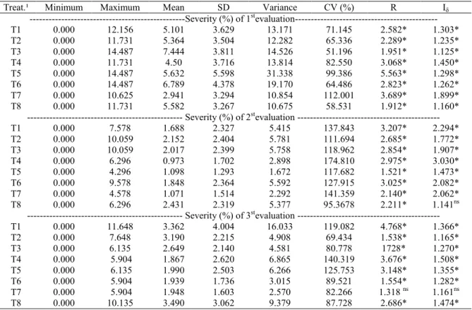
Table 2. Minimum and maximum values, mean, standard deviation (SD), variance, coefficient of variation (CV) variance, mean ratio (R), and Morisita index (Iδ) of blast’s severity, and area under the disease progress curve, in experiment 1.

* Randomness rejected at 5% probability of error. ns_{Randomness is not rejected. ¹Treatments described in details in}

Table 1. –Values not calculated.

Treat.¹ Minimum Maximum Mean SD Variance CV (%) R Iδ

---Severity (%) of 1stevaluation--- T1 0.000 12.156 5.101 3.629 13.171 71.145 2.582* 1.303* T2 0.000 11.731 5.364 3.504 12.282 65.336 2.289* 1.235* T3 0.000 14.487 7.444 3.811 14.526 51.196 1.951* 1.125* T4 0.000 11.731 4.50 3.716 13.814 82.550 3.068* 1.450* T5 0.000 14.487 5.632 5.598 31.338 99.386 5.563* 1.298* T6 0.000 14.487 6.789 4.378 19.170 64.486 2.823* 1.262* T7 0.000 10.625 2.941 3.294 10.854 112.001 3.689* 1.899* T8 0.000 11.731 5.582 3.267 10.675 58.531 1.912* 1.160*

--- Severity (%) of 2stevaluation --- T1 0.000 7.578 1.688 2.327 5.415 137.843 3.207* 2.294* T2 0.000 10.059 2.152 2.404 5.781 111.694 2.685* 1.772* T3 0.000 10.059 2.017 2.399 5.758 118.962 2.854* 1.907* T4 0.000 6.296 0.973 1.702 2.898 174.810 2.975* 3.030* T5 0.000 4.296 1.098 1.293 1.672 117.682 1.521* 1.473* T6 0.000 9.578 1.848 2.364 5.592 127.915 3.025* 2.082* T7 0.000 4.578 1.071 1.514 2.292 141.359 2.140* 2.062* T8 0.000 6.296 2.431 2.319 5.377 95.3678 2.211* 1.141ns

(5)

Rev. Caatinga

Table 2. Continuation.

*Randomness rejected at 5% probability of error. ns_{Randomness is not rejected. ¹Treatments described in details in}

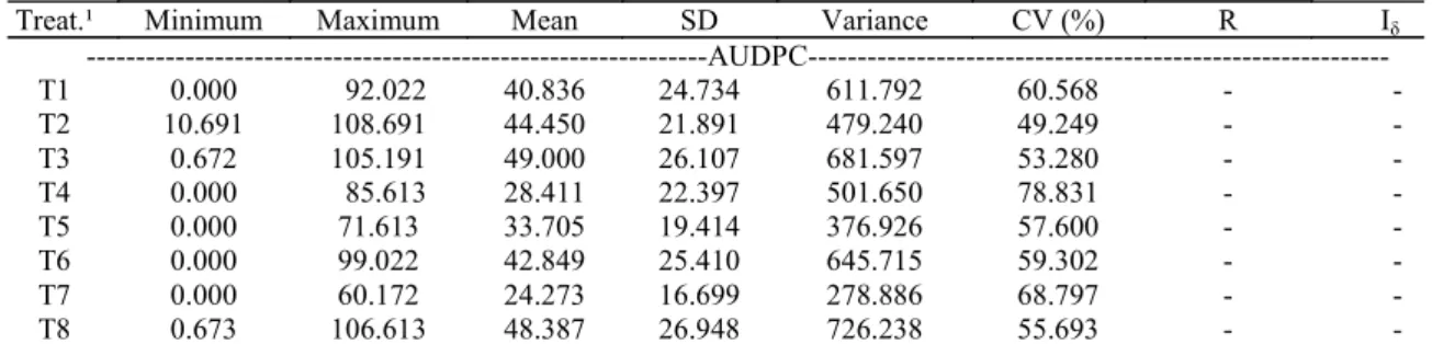
Table 3. Minimum and maximum values, mean, standard deviation (SD), variance, coefficient of variation (CV) variance, mean ratio (R), and Morisita index (Iδ) of blast’s severity, and area under the disease progress curve, in experiment 2.

* Randomness rejected at 5% probability of error. ns_{Randomness is not rejected. ¹Treatments described in details in}

Treat.¹ Minimum Maximum Mean SD Variance CV (%) R I_δ ---AUDPC--- T1 0.000 92.022 40.836 24.734 611.792 60.568 - - T2 10.691 108.691 44.450 21.891 479.240 49.249 - - T3 0.672 105.191 49.000 26.107 681.597 53.280 - - T4 0.000 85.613 28.411 22.397 501.650 78.831 - - T5 0.000 71.613 33.705 19.414 376.926 57.600 - - T6 0.000 99.022 42.849 25.410 645.715 59.302 - - T7 0.000 60.172 24.273 16.699 278.886 68.797 - - T8 0.673 106.613 48.387 26.948 726.238 55.693 - -

Treat.¹ Minimum Maximum Mean SD Variance CV (%) R I_δ ---Severity (%) of 1st_{evaluation---}

T1 1.619 13.752 5.575 2.416 5.838 43.341 1.047ns 1.008 ns T2 1.752 14.275 7.425 2.812 7.910 37.880 1.065 ns _1.008 ns

T3 0.752 9.352 5.525 2.122 4.507 38.424 1.033 ns 0.967 ns T4 8.710 12.845 10.300 3.673 13.491 55.442 2.036* 1.153* T5 0.000 16.352 6.699 3.927 15.426 58.627 2.302* 1.190* T6 2.275 16.752 7.250 3.637 13.229 50.168 1.824* 1.111* T7 2.752 11.352 6.800 2.402 5.769 35.324 0.848 ns 0.978 ns T8 1.752 12.619 7.400 2.687 7.224 36.321 0.976 ns _0.996 ns

T9 3.352 19.275 11.025 4.962 24.622 45.007 1.825* 1.073* --- Severity (%) of 2st_{evaluation ---}

T1 8.710 13.314 10.360 1.134 1.287 10.951 0.124 ns 0.917 ns T2 8.710 13.314 10.390 1.528 2.336 14.707 0.224 ns _0.919 ns

T3 9.130 12.710 10.275 0.864 0.746 8.409 0.072 ns 0.911 ns T4 8.710 12.845 10.300 0.959 0.921 9.318 0.089 ns _0.913 ns

T5 8.814 14.130 10.705 1.278 1.634 11.943 0.152 ns 0.922 ns T6 8.710 12.314 10.275 0.981 0.963 9.552 0.093 ns _0.913 ns

T7 8.710 13.814 11.070 1.215 1.476 10.976 0.133 ns 0.923 ns T8 9.130 14.130 10.787 0.960 0.922 8.902 0.085 ns _0.917 ns

T9 9.210 16.710 12.162 1.717 2.950 14.122 0.503 ns 0.939 ns --- Severity (%) of 3st_{evaluation ---}

T1 2.515 21.715 10.013 4.901 24.024 239.913 1.767* 1.074* T2 2.715 32.515 13.150 7.620 58.075 57.952 4.416* 1.253* T3 3.248 34.715 14.575 7.876 62.044 54.043 4.256* 1.178* T4 1.715 22.515 10.362 4.790 22.944 46.224 2.214* 1.114* T5 3.515 35.748 15.675 10.475 109.733 66.828 7.001* 1.302* T6 0.000 35.748 13.187 8.090 65.464 61.355 4.964* 1.293* T7 2.748 29.715 14.350 6.889 47.461 48.008 3.307* 1.157* T8 14.715 40.748 27.800 7.860 61.787 28.275 2.222* 1.042* T9 9.515 32.515 17.050 7.457 55.611 43.737 1.450* 1.025*

(6)

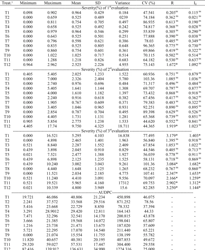
Table 4. Minimum and maximum values, mean, standard deviation (SD), variance, coefficient of variation (CV) variance, mean ratio (R), and Morisita index (Iδ) of blast’s severity, and area under the disease progress curve, in experiment 3.

*Randomness rejected at 5% probability of error. ns_{Randomness is not rejected. ¹Treatments described in details in}

The assumptions of the mathematical model were not met in case of the disease severity variable and therefore the non-parametric Friedman test was carried out to compare the severity of the treatments for the three evaluations. In the case of the AUDPC variable, the assumptions have been met, since the transformation of the variable in experiments 2 and 3

was required. The Friedman test showed that the severity of the disease was not the same in all treatments (p-value <0,05). Moreover, the difference in AUDPC values emphasized the difference in the progress of the disease among the fungicide treatments (Table 5).

Treat.¹ Minimum Maximum Mean SD Variance CV (%) R I_δ ---Severity(%) of 1st_{evaluation---}

T1 0.098 0.902 0.964 0.429 0.184 47.541 0.203ns 0.115 ns T2 0.000 0.659 0.525 0.489 0239 74.184 0.362 ns 0.021 ns T3 0.000 0.811 0.754 0.705 0.497 86.935 0.613 ns 0.190 ns T4 0.000 0.658 0.525 0.492 0.242 74.817 0.368 ns _0.028 ns

T5 0.000 0.979 0.964 0.546 0.299 55.839 0.305 ns 0.290 ns T6 0.000 0.643 0.525 0.501 0.251 77.888 0.390 ns 0.038 ns T7 0.000 0.796 0.598 0.621 0.386 78.03 0.485 ns 0.349 ns T8 0.000 0.835 0.525 0.805 0.648 96.365 0.775 ns _0.730 ns

T9 0.000 0.860 0.754 0.601 0.361 69.866 0.419 ns 0.322 ns T10 0.000 1.022 1.025 0.717 0.514 70.115 0.502 ns 0.514 ns T11 0.000 1.288 1.218 0.826 0.683 64.182 0.530 ns 0.637 ns T12 0.964 2.962 2.525 2.226 4.955 75.143 1.672* 1.092 ns

--- Severity (%) of 2stevaluation --- T1 0.405 5.405 2.025 1.233 1.522 60.936 0.751 ns 0.879 ns T2 0.000 7.000 2.326 2.404 5.780 103.36 1.085 ns 1.036 ns T3 0.000 2.740 0.976 0.696 0.484 71.317 0.496 ns _0.484 ns

T8 0.000 3.405 1.046 0.965 0.931 92.251 0.890 ns 0.895 ns T9 0.000 2.854 0.787 0.704 0.495 89.398 0.629 ns _0.526 ns

T10 0.000 4.405 1.731 1.131 1.281 65.368 0.739 ns 0.851 ns T11 0.905 5.854 2.775 1.238 1.533 44.620 0.552 ns _0.841 ns

T12 4.405 17.74 9.750 4.325 18.711 44.365 1.919* 1.023 ns --- Severity (%) of 3stevaluation --- T1 0.000 16.521 5.295 4.103 16.838 77.495 3.179* 1.403* T2 0.000 4.898 2.465 1.401 1.963 56.840 1.395 ns _0.918 ns

T7 0.439 10.240 3.002 3.043 9.261 101.36 3.084* 1.682* T8 0.000 4.440 1.648 1.125 1.265 68.232 0.767 ns _0.860 ns

T9 0.000 11.521 2.034 2.185 4.775 107.41 2.347* 1.653* T10 0.521 11.240 4.410 3.091 9.556 70.097 2.166* 1.259* T11 0.521 19.521 5.965 4.160 17312 69.753 2.902* 1.312* T12 0.021 10.339 4.800 3.949 15.6 82.285 3.250* 1.144*

(7)

Rev. Caatinga

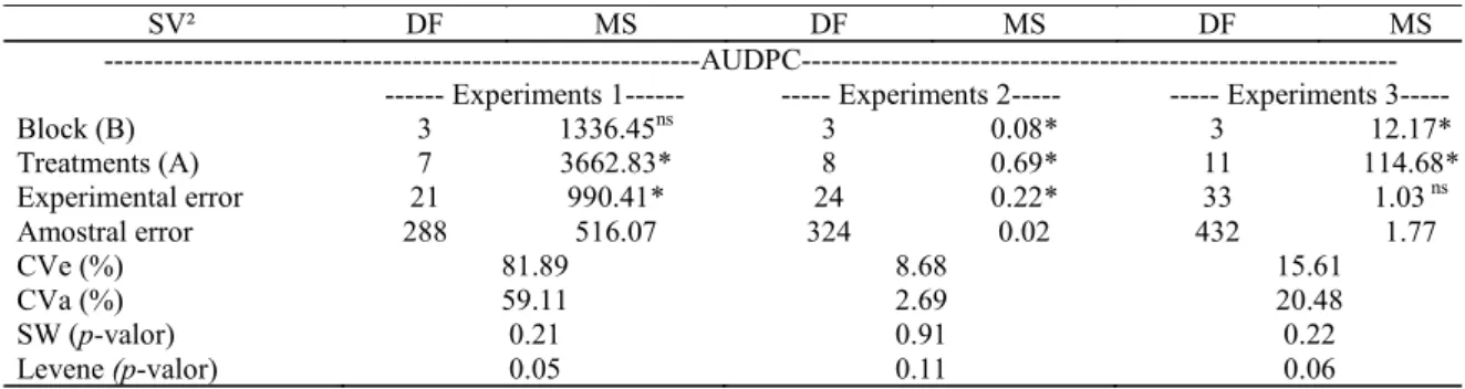
Table 5. Summary of the analysis of variance (ANOVA) of the three experiments for the area under the disease progress curve (AUDPC).

SV² DF MS DF MS DF MS

---AUDPC--- --- Experiments 1--- --- Experiments 2--- --- Experiments 3--- Block (B) 3 1336.45ns 3 0.08* 3 12.17* Treatments (A) 7 3662.83* 8 0.69* 11 114.68* Experimental error 21 990.41* 24 0.22* 33 1.03 ns Amostral error 288 516.07 324 0.02 432 1.77

CVe (%) 81.89 8.68 15.61

CVa (%) 59.11 2.69 20.48

SW (p-valor) 0.21 0.91 0.22

Levene (p-valor) 0.05 0.11 0.06

*Significant effect by the F test at 5% error probability; :ns_{Not significant effect according to the F test at 5% error}

probability. ¹Experiments described in details in Table 1; ²SV = Sources of variation; DF = degrees of freedom; MS = Mean square; CVa = coefficient of variation of the amostral error; CVe = coefficient of variation of the experimental error; SW ( p-value) = pvalue of the Shapiro-Wilk normality test; Levene (p-value) = pvalue of the homogeneity test of Levene variances.

In experiments 1 and 2, the residual and sample variances were heterogeneous between each other and the variability between plots (residual) was greater than the variability within plots (sample), indicating that the experimental error was greater than the sampling error (Table 5). The values of the coefficient of variation of higher sampling errors reinforced that the variability between plots was greater than within plots, and reveal the need to resize the experiments in terms of the number of repetitions. However, the high value of the coefficient of variation by analysis of variance of experimental and amostral error, especially in experiment 1, indicates low precision and reinforces the need for resizing the experiments by increasing the number of repetitions and sample size (CARGNELUTTI FILHO et al., 2008; CARGNELUTTI FILHO et al., 2009; KRAUSE et al., 2013).

The high experimental error leads to an increased mean square of the experimental error, hindering the H0 rejection of the hypothesis and

raising possibility of Type II error (STORCK et al., 2006). Thus, the number of repetitions must be increased along with proper sizing of the sample size, which could contribute to reduced experimental error and thus obtain more precise conclusions (CARGNELUTTI FILHO et al., 2008; CARGNELUTTI FILHO et al.,2009; KRAUSE et al, 2013).

Variances of the data observed were heterogeneous between treatments, both for severity and AUDPC variable, in all experiments. The heterogeneity of variances of the data observed between assessments was observed in 79,41% of the treatments. The difference in blast’s severity, disease progress (determined by AUDPC) between treatments, heterogeneity of variances of the data observed between treatments and evaluations showed that the 40 leaves evaluated in each treatment should be considered as an independent sample. Therefore, we chose to determine the sample

size required to evaluate the severity of the blast and AUDPC for each treatment and assessment, separately.

The variability observed in field experiments is usually attributed to environmental factors, soil variability, or genetic factors (MARTIN et al., 2005; CARGNELUTTI FILHO et al., 2009; LÚCIO et al., 2009). However, in the case of diseases, factors such as the spread of the disease on the field must also be taken into consideration (MICHEREFF et al., 2011). To obtain an optimal sample size, different conditions are desirable so that the recommendation is not so limited. In case of diseases, sampling practices should be considered among the different field conditions, since disease spread and, therefore, sample size may vary according to the year, sowing time, cultivation site, and time of evaluation (SILVA et al., 2008; MICHEREFF et al., 2008; MICHEREFF et al., 2011).

The interpretation of the values referring to the average coefficient of variation of blast severity and area under the disease progress curve variables (Table 2, 3 and 4) is indicative of the variation between the leaves evaluated and, thus, the sample size (STURMER et al., 2013). The larger the coefficient of variation, the greater the dispersion of the observations around the average, suggesting the need for a larger number of samples (number of flagged leaves) for more accurate estimation. Based on these values, the tendency of the sample size to be higher for the estimation of blast’s severity in relation to AUDPC was observed.

(8)

aggregated, the size of the sample is calculated by

the equation , where k is a parameter associated with the negative binomial distribution, describing the aggregated arrangement of infected plants. According to the same authors, infected plants spread randomly in the field follow the Poisson distribution, which is characterized by

. In this case, the equation used to calculate

the sample size is . Finally, when the dispersion of the disease is not the same over time or between treatments, as in this study, the recommended formula to determine the sample size

is , which many authors refer to as undetermined distribution. In our experiments, the dispersion of leaf blast was dependent on the treatment and the time of evaluation. The type of distribution of the disease was not the same throughout the experiment, indicating that the method used to calculate the sample size in this

2 2

2 / ) (

x CV k x

z x k n  

2

s

x

2 2

2 /

x CV x

z n 

2 2

) 2 / (

x CV x

s z n 

study was suitable.

The sample size for the average estimation of blast’s severity was different among treatments and evaluations. This behavior was expected, since the difference observed in the average severity of treatments and evaluations, as well as the heterogeneity of variances between treatments and evaluations in each treatment, leads to changes in the ratio between variance and variables average values. This ratio is indicative of disease spread in the field, which affects the sample size, and this relationship was included in the methodology used. Thus, three sample sizes per treatment (one evaluation) were estimated for this variable, with only the largest presented in Table 6.

In case of AUDPC, only one sample size was determined per treatment. It was observed that the tendency to reduce the number of flagged leaves evaluated when using the AUDPC variable in relation to severity variable. AUDPC is widely used in phytopathological studies, as it characterizes the interaction between the pathogen, the environment and the host, in addition to being used as a form of evaluation of control strategies (BERGAMIN FILHO, 1997).

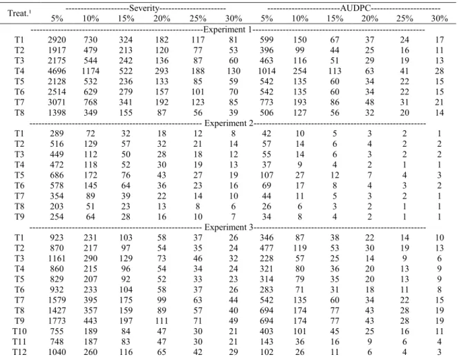
Table 6. Sample size, given as expressed as number of flagged leaves per plot, to estimate the average severity and area under the disease progress curve (AUDPC) of the blast in the three experiments analyzed.

¹Treatments described in details in Table 1.

Treat.¹ ---Severity--- ---AUDPC--- 5% 10% 15% 20% 25% 30% 5% 10% 15% 20% 25% 30% ---Experiment 1--- T1 2920 730 324 182 117 81 599 150 67 37 24 17 T2 1917 479 213 120 77 53 396 99 44 25 16 11 T3 2175 544 242 136 87 60 463 116 51 29 19 13 T4 4696 1174 522 293 188 130 1014 254 113 63 41 28 T5 2128 532 236 133 85 59 542 135 60 34 22 15 T6 2514 629 279 157 101 70 542 135 60 34 22 15 T7 3071 768 341 192 123 85 773 193 86 48 31 21 T8 1398 349 155 87 56 39 506 127 56 32 20 14

--- Experiment 2--- T1 289 72 32 18 12 8 42 10 5 3 2 1 T2 516 129 57 32 21 14 57 14 6 4 2 2 T3 449 112 50 28 18 12 55 14 6 3 2 2 T4 472 118 52 30 19 13 37 9 4 2 1 1 T5 686 172 76 43 27 19 107 27 12 7 4 3 T6 578 145 64 36 23 16 69 17 8 4 3 2 T7 354 89 39 22 14 10 44 11 5 3 2 1 T8 203 51 23 13 8 6 26 6 3 2 1 1 T9 254 64 28 16 10 7 34 8 4 2 1 1

(9)

Rev. Caatinga

It is observed that the number of leaves to be evaluated in order to estimate the severity (percentage of the attacked tissue) of the blast is greater than the number used to estimate AUDPC. The smaller number of leaves required to estimate AUDPC is mainly related to the reduction of the effect of null values (zeros) in the database. Inflation of zeros in the database is the result of the absence of symptoms in some leaves that were sampled while others present symptoms. The presence of null values increases the variability of the data, requiring more extensive sampling to estimate the average severity of the disease.

For an acceptable error of 5%, the sample size required to estimate the average severity of blast is of 4696 flag leaves. As for AUDPC variable, the number of leaves that needs to be evaluated is 1014 (Table 6). The evaluation of this number of leaves becomes impractical, due to the amount of labor and time required. Therefore, it is recommended to use larger sample sizes with greater pre-established errors. Furthermore, the use of the variable AUDPC is recommended whenever possible, as a means of comparison between treatments. Therefore, for an error of 20% and confidence level of 95%, the evaluation of 63 flag leaves is necessary to estimate AUDPC, a more common form of quantification of the disease in works in the plant pathology field. If an experiment is formed of 4 repetitions, it is necessary to evaluate 16 leaves per plot.

The greater the precision required the more the leaves that should be evaluated. The accuracy of the estimate and, subsequently, the sample dimension should be left to the researcher, as the ideal sample size will depend on the minimum acceptable error in every situation (type of study) as well as the labor and resources available to each researcher (MICHEREFF et al., 2008; MICHEREFF et al., 2011; TOEBE et al., 2011; STÜRMER et al., 2013).

CONCLUSION

A variability of the sample size was observed in the evaluation of leaf blast, according to the treatments used and type of evaluations carried out over time. The sample size required to estimate the average area under the blast progress curve is smaller than that to assess severity. For an acceptable error of 20%, the sample size per plot required to estimate the average severity of the blast is 293 flag leaves and for the variable AUDPC, the number of flag leaves to be evaluated is 63.

REFERENCES

BEDENDO, I. P. Doenças do Arroz. In: KIMATI, H.

et al. (Eds.). Manual de Fitopatologia: Doenças em plantas cultivadas. São Paulo: Ceres, 1997. v. 2, cap. 33 p. 88-102.

BERGAMIN FILHO, A. Avaliação de danos e perdas. In: KIMATI, H. et al. (Eds.). Manual de Fitopatologia: Princípios e conceitos. São Paulo: Ceres, 1997. v. 1, cap. 10, p. 672-690.

CAMPBELL, C. L.; MADDEN, L. V. Introduction to plant disease epidemiology. New York: John Willey, 1990. 532 p.

CARGNELUTTI FILHO, A. et al. Tamanho de amostra de caracteres de genótipos de soja. Ciência Rural, Santa Maria, v. 39, n. 4, p. 983-991, 2009.

CARGNELUTTI FILHO, A. et al. Tamanho de amostra de caracteres de cultivares de feijão. Ciência Rural, Santa Maria, v. 38, n. 3, p. 635-642, 2008.

CATAPATTI, T. R. et al. Tamanho de amostra e número de repetições para a avaliação de caracteres agronômicos em milho-pipoca. Ciência e Agrotecnologia, Lavras, v. 32, n. 3, p. 855-862, 2008.

CELMER, A. et al. Controle químico de doenças foliares na cultura do arroz irrigado. Pesquisa Agropecuária Brasileira, Brasília, v. 42, n. 6, p. 901-904, 2007.

COUNCE, P. A.; KEISLING, T. C.; MITCHELL, A. J. A uniform, objective, and adaptative system for expressing rice development. Crop Science, Madison, v. 40, n. 2, p. 436-443, 2000.

FILIPPI, M. C. C. Indução de resistência à brusone em folhas de arroz por isolado avirulento de Magnaporthe oryzae. Fitopatologia Brasileira, Brasília, v. 32, n. 5, p. 387-392, 2007.

IRRI. INTERNATIONAL RICE RESEARCH INSTITUTE. Standard evaluation system of rice (SES). Manila: IRRI, 2002. 4 ed. 56 p.

KRAUSE, W. et al. Tamanho ótimo de amostra para avaliação de caracteres de frutos de abacaxizeiro em experimentos com adubação usando parcelas grandes. Revista Brasileira de Fruticultura, Jaboticabal, v. 35, n. 1, p. 183-190, 2013.

LÚCIO, A. D. et al. Distribuição espacial e tamanho de amostra para o ácaro-bronzeado da erva-mate. Revista Árvore, Viçosa, v. 33, n. 1, p. 143-150, 2009.

(10)

MICHEREFF, S. J. et al. Sample size for quantification of cercospora leaf spot in sweet pepper. Journal of Plant Pathology, Bari, v. 93, n. 1, p.83-186, 2011.

MICHEREFF, S. J.; NORONHA, M. A.; MAFFIA, L. A. Tamanho de amostras para avaliação da severidade da queima das folhas do inhame. Summa Phytopathologica, Botucatu, v. 34, n. 2, p. 189-191, 2008.

PRABHU, A. S. et al. Estimativa de danos causados pela brusone na produtividade de arroz de terras altas. Pesquisa Agropecuária Brasileira, Brasília, v. 38, n. 9, p. 1045-1051, 2003.

R DEVELOPMENT CORE TEAM. R: A Language and Environment for Statistical Computing. R Foundation for Statistical Computing, Vienna, Áustria. 2012.

SANTOS, G. R. et al. Fungicidas para o controle das principais doenças do arroz irrigado. Biosciense Journal, Uberlândia, v. 25, n. 4, p. 11-18, 2009.

SILVA, A. M. F. et al. Tamanho de amostras para quantificação da podridão-mole da alface e da couve-chinesa. Summa Phytopathologica, Botucatu, v. 34, n. 1, p. 90-92, 2008.

SILVA, E. I. et al. Levantamento da incidência da mancha-aquosa do melão no Rio Grande do Norte e determinação do tamanho das amostras para quantificação da doença. Summa Phytopathologica, Botucatu, v. 29, n. 2, p. 172-176, 2003.

SOSBAI - SOCIEDADE SUL-BRASILEIRA DE

ARROZ IRRIGADO. Arroz irrigado: recomendações técnicas da pesquisa para o Sul do

Brasil. 1. ed. Pelotas, RS: SOSBAI, 2007. 154 p.

STORCK, L. et al. Experimentação vegetal. 2. ed. Santa Maria, RS: UFSM, 2006. 198 p.

STURMER, G. R. et al. Tamanho de amostra para a estimação da média de lagartas na cultura de soja. Biosciense Journal, Uberlândia, v. 29, Sup. 1, p. 1596-1605, 2013.