LUÍS MANUEL TREMOCEIRO BAPTISTA

LUÍS MANUEL TREMOCEIRO BAPTISTA

U

SING

R

ESTARTS IN

C

ONSTRAINT

P

ROGRAMMING OVER

F

INITE

D

OMAINS

AN EXPERIMENTAL EVALUATION

Dissertação para obtenção do Grau de Doutor em Informática

Orientador: Francisco de Moura e Castro Ascensão de Azevedo,

Professor Auxiliar da Faculdade de Ciências e Tecnologia da

Universidade NOVA de Lisboa

Júri

Presidente: Prof. Doutor Pedro Manuel Corrêa Calvente Barahona Arguentes: Prof. Doutor Christophe Lecoutre

Prof. Doutor Mikoláš Janota

Vogais: Prof. Doutora Ana Paula Tomás

Prof. Doutor Francisco de Moura e Castro Ascensão de Azevedo Prof. Doutor José Carlos Ferreira Rodrigues da Cruz

Doutor Marco Vargas Correia

Using Restarts in Constraint Programming over Finite Domains - An Experimental

Evaluation

Copyright © Luís Manuel Tremoceiro Baptista, Faculdade de Ciências e Tecnologia, Universidade Nova de Lisboa

A

CKNOWLEDGEMENTS

To my supervisor, Professor Francisco Azevedo, for the valuable support and perseverance, especially when good results did not appear. I am thankful that he managed to find the necessary funding that allowed me to attend important conferences. And also, to participate in a summer school, where I was introduced and trained with the Comet System, which I used in this PhD Thesis. I also thank Marco Correia for explaining how the CaSPER Constraint Solver works, although I have not used it.

To my School of Technology and Business Studies of the Polytechnic Institute of Portalegre, which gave me all the possible support, among the fewer available. Particularly, I want to thank to my colleague and friend Paulo Brito for all the support and encouragement. Also, the work presented in this Thesis was partially supported by the Portuguese “Fundação para a Ciência e a Tecnologia” (SFRH/PROTEC/49859/2009).

A

BSTRACT

The use of restart techniques in complete Satisfiability (SAT) algorithms has made solving hard real world instances possible. Without restarts such algorithms could not solve those instances, in practice. State of the art algorithms for SAT use restart techniques, conflict clause recording (nogoods), heuristics based on activity variable in conflict clauses, among others. Algorithms for SAT and Constraint problems share many techniques; however, the use of restart techniques in constraint programming with finite domains (CP(FD)) is not widely used as it is in SAT. We believe that the use of restarts in CP(FD) algorithms could also be the key to efficiently solve hard combinatorial problems.

In this PhD thesis we study restarts and associated techniques in CP(FD) solvers. In particular, we propose to including in a CP(FD) solver restarts, nogoods and heuristics based in nogoods as this should improve search algorithms, and, consequently, efficiently solve hard combinatorial problems.

We thus intend to: a) implement restart techniques (successfully used in SAT) to solve constraint problems with finite domains; b) implement nogoods (learning) and heuristics based on nogoods, already in use in SAT and associated with restarts; and c) evaluate the use of restarts and the interplay with the other implemented techniques.

We have conducted the study in the context of domain splitting backtrack search algorithms with restarts. We have defined domain splitting nogoods that are extracted from the last branch of the search algorithm before the restart. And, inspired by SAT solvers, we were able to use information within those nogoods to successfully help the variable selection heuristics. A frequent restart strategy is also necessary, since our approach learns from restarts.

R

ESUMO

A utilização de técnicas de restarts em algoritmos completos para Solvabilidade

Proposicional (SAT) tornou possível a resolução de problemas reais difíceis, que na prática não conseguiam ser resolvidos sem restarts. Os melhores algoritmos de SAT

usam técnicas de restarts, registo de cláusulas de conflito (nogoods), heurísticas baseadas

na atividade de variáveis nas cláusulas de conflito, entre outras técnicas. Os algoritmos para SAT e para programação por restrições sobre domínios finitos (CP(FD)) partilham muitas técnicas; no entanto, em CP(FD) os restarts não são usados de forma tão alargado

como em SAT. Pensamos que a utilização de restarts em algoritmos para CP(FD) pode

também ser a chave para resolver de forma mais eficiente problema combinatórios difíceis.

Nesta tese de doutoramento estudamos em CP(FD) os restarts e técnicas associadas.

Em particular, propomos implementar os restarts, nogoods e heurísticas baseadas em nogood, de forma a melhorar o algoritmo de procura e, consequentemente, resolver de

forma eficiente problemas combinatórios difíceis.

Assim, pretendemos: a) implementar técnicas de restarts (utilizadas com sucesso em

SAT) para resolver problemas de restrições sobre domínios finitos; b) implementar

nogoods (aprendizagem automática) e heurísticas baseadas nesses nogoods, já utilizadas

em SAT e associadas a restarts; e c) avaliar o uso de restarts e a sua interação com outras

técnicas implementadas.

Este estudo foi levado a cabo no contexto dos algoritmos de procura com retrocesso, utilizando restarts, e com domain splitting (ds). Definimos nogoods que são extraídos do

último ramo da árvore de procura antes do restart. Inspirados pelos algoritmos de SAT,

conseguimos usar informação contida nos nogoods para ajudar a heurística de seleção de

variável. É necessário uma política de restarts frequentes, uma vez que a nossa

abordagem aprende com os restarts.

Palavras-chave: restarts; nogoods; heurísticas; Programação por restrições; procura

C

ONTENTS

1 Introduction ... 1

1.1 General Overview ... 1

1.2 Challenges and Contributions ... 2

1.3 Thesis Map ... 5

2 Constraint Solving ... 7

2.1 Constraint Satisfaction Problem ... 7

2.1.1 Definitions ... 7

2.1.2 Search algorithms ... 9

2.1.3 Branching schemes ... 11

2.1.4 Learning ... 12

2.1.5 Examples of CSP Problems ... 14

2.2 Satisfiability Problems ... 23

2.2.1 Definition ... 23

2.2.2 Search Algorithms... 25

2.3 Summary and Final Remarks ... 28

3 Heuristics ... 29

3.1 Static versus dynamic variable ordering heuristics ... 30

3.2 The fail first principle ... 31

3.3 Weighted based (Conflict-driven) heuristic ... 34

3.4 Other state of the art heuristics ... 36

3.5 Sat heuristics ... 38

3.6 Summary and Final Remarks ... 40

4 Restarts ... 43

4.1 Randomization and Heavy-tail ... 45

4.2 Search restart strategies ... 47

4.3 Completeness ... 49

4.4 Learning from restarts ... 50

4.5 Results on Restarts ... 53

4.5.1 Preliminary results ... 53

4.5.2 Using Restarts ... 57

4.5.3 Difficulties on using restarts ... 61

4.6 Summary and Final Remarks ... 62

5 Domain-Splitting Nogoods ... 65

5.1 Simplifying ds-nogoods ... 68

5.2 Generalizing to dsg-nogoods ... 70

5.3 Posting ds-nogoods ... 71

5.4 Summary and Final Remarks ... 76

6 Using Ds-Nogoods in Heuristics ... 79

6.1 Trying information from ds-nogoods ... 81

6.2 Ds-nogood-based heuristic ... 85

6.3 Results on ds-nogood based heuristic ... 87

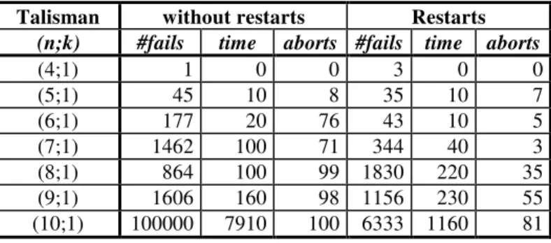
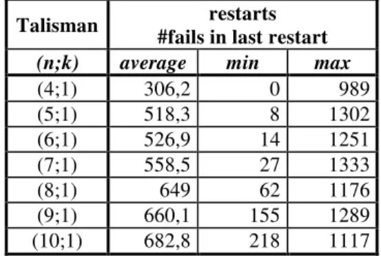
6.3.1 Talisman squares ... 89

6.3.2 Latin Squares ... 90

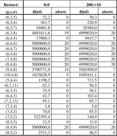
6.3.3 Restart strategies ... 91

C

6.4.1 Flexible Domain-splitting branching ... 96

6.4.2 Importance of domain-splitting branching ... 102

6.5 Comparing with dom/wdeg ... 104

6.5.1 Importance of domain splitting branching with dom/wdeg ... 109

6.6 Trying to improve dom/wdeg ... 110

6.7 Summary and Final Remarks ... 114

7 Conclusions and Future Work... 117

L

IST OF

F

IGURES

Fig. 2.1. Example of different branching schemes ... 12

Fig. 2.2. Example of n-queens problem ... 15

Fig. 2.3. Comet model for N-Queens... 16

Fig. 2.4. Example of a Magic Square ... 17

Fig. 2.5. Comet model for Magic square ... 18

Fig. 2.6. Extra constraints for the Talisman square Comet model ... 18

Fig. 2.7. Example of Latin squares ... 19

Fig. 2.8. Comet model for Latin square ... 19

Fig. 2.9. Comet Model for Golfers (without symmetries) ... 20

Fig. 2.10. Comet model for Prime queen ... 21

Fig. 2.11. Partial Comet model for Cattle Nutrition ... 22

Fig. 4.1. 8-queens heavy-tail distribution ... 46

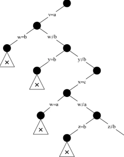
Fig. 4.2. Partial search tree before the restart, with 2-way branching. ... 51

Fig. 5.1 Partial search tree before the restart, with domain-splitting branching ... 66

Fig. 5.2 Distribution of ds-nogoods sizes for Talisman squares ... 74

L

IST OF

T

ABLES

Table 4.1. Number of backtracks to solve different n-queens instances ... 55

Table 4.2. Number of backtracks for the conflict-driven heuristic ... 56

Table 4.3. Average number of fails, runtime and aborts, for 100 runs... 58

Table 4.4. Minimum number of fails, runtime and aborts, for 100 runs ... 58

Table 4.5. Number of fails in the last restart of each run ... 59

Table 4.6. Average number of fails, runtime and aborts, for 100 runs of latin squares ... 60

Table 4.7. Using restarts on Golfers ... 62

Table 5.1. Ds-Nogoods size for Talisman square instances ... 73

Table 5.2. Ds-Nogoods size for Latin square instances ... 74

Table 5.3. Relation between ds-nogoods sizes and maximum size ... 76

Table 6.1 Average Number of Fails, Runtime and Aborts, for 100 Runs ... 89

Table 6.2 Average Number of Fails, Runtime and Aborts, for 100 Runs of Latin Squares ... 91

Table 6.3 Comparing Different Restart Strategies ... 92

Table 6.4. Average Number of Fails and Aborts, for 100 Runs (v2) ... 97

Table 6.5. Comparing Talisman Square ds-splitting flex ... 98

Table 6.6. Average Number of Fails and Aborts, for 100 Runs of Latin Squares (v2) .... 99

Table 6.7. Average Number of Fails and Aborts, for 100 Runs of Talisman Squares (Original) ... 100

Table 6.8. Average Number of Fails and Aborts, for 100 Runs of Magic Squares ... 101

Table 6.10. Average Number of Fails and Aborts, for 100 Runs of Talisman Squares

(Original, 2-way) ... 103

Table 6.11. Latin square with dom/wdeg ... 106

Table 6.12. Magic square with dom/wdeg ... 106

Table 6.13. Talisman square with dom/wdeg ... 107

Table 6.14. Original Talisman square with dom/wdeg ... 108

Table 6.15. Golfers with dom/wdeg ... 108

Table 6.16. Comparing dom/wdeg heuristics in branching ... 110

Table 6.17. Comparing heuristics ... 112

Table 6.18. Comparing Latin square with dom/wdeg+act ... 113

1

I

NTRODUCTION

1.1

G

O

Constraint Satisfaction Problems (CSPs) are a well-known case of NP-complete problems (Apt, 2003). They have extensive application in areas such as scheduling, configuration, timetabling, resources allocation, combinatorial mathematics, games and puzzles, and many other fields of computer science and engineering.

One of the major progress of backtrack search algorithms for SAT was the combined use of restarts and nogood recording (learning) (Baptista and Silva, 2000), and also the use of efficient data structures and an heuristic based on the learned nogoods (Moskewicz et al., 2001). Because these techniques are not widely used in backtrack search algorithms for CP(FD), and because the two areas (CP(FD) and SAT) have mutually benefited with the progress of each other (Bordeaux et al., 2006), we propose to study the interplay of those techniques in the context of CP(FD).

In backtrack search algorithms different branching schemes could be used, e.g., d-way and 2-d-way are the most traditional and widely used. But in our study we focus on domain splitting branching scheme (Dincbas et al., 1988), using restarts and nogood recording from restarts. From the empirical study we found a way of using information from nogoods in the variable selection heuristic. In fact, that information really improves the fail-first heuristic and, although not with the same impact, it could improve the state-of-the-art conflict failure dom/wdeg heuristic.

In some classes of problems we found that the joint use of restarts, nogoods and heuristics have shown improvements of the algorithms. In fact, when studying the interplay of restarts strategies, heuristics and nogoods from restarts in CP(FD) algorithms, we do not see improvements when using restarts per se, nor when adding nogoods; but,

when adding a third component, heuristics using information from nogoods, promising results can be achieved. As it happens in SAT algorithms these joint use of techniques could also be the key to improve CP(FD) algorithms, which seems to be a promising line of research.

1.2

C

C

1.2

C

C

use of variable and value selection heuristics, e.g., based on the fail-first principle (Haralick and Elliott, 1979), is of great importance for efficiently solving CSPs. On the contrary, the use of restart techniques is not widely used in backtrack search algorithms for solving CP(FD) as it is in SAT.

A known problem in backtrack search algorithms, due to bad choices near the root of the search tree, is the extreme computational effort needed, because of the combinatorial explosion of the search space. Avoiding being trapped in an unpromising search sub-tree is critical to the success of backtrack search algorithms. It is possible to jump to other parts of the search tree, restarting the search, in non-deterministic cycles, until a solution is found (Gomes et al., 1998).

Restarts have been used to successfully solve hard real world satisfiability problems (SAT) (Baptista and Silva, 2000; Moskewicz et al., 2001). Restart techniques require the use of a randomized algorithm, typically randomizing decision heuristics, and the use of nogoods recording (generically known as learning and, in the context of SAT, as clause recording). Simple decision heuristics, based on conflicts, have shown to be more competitive (Moskewicz et al., 2001). The use of nogoods improves the overall performance of backtrack search algorithms, since it avoids bad past decisions to be made again. Aborting the search and restarting again makes the resulting algorithm incomplete; however, various strategies exist that make the algorithm complete (Baptista et al., 2001; Baptista and Silva, 2000; Lecoutre et al., 2007a; Mehta et al., 2009; Walsh, 1999).

The relationship between SAT and CP(FD) areas is high (Bordeaux et al., 2006). Both are used to model and solve decision problems, i.e., both have variables and constraints over the variables, and the goal is to find an assignment to all the variables, such that all the constraints are satisfied. Both use complete or incomplete search algorithms, to solve the problem. Even algorithmic techniques used in both areas are similar. Also, the two areas have mutually benefited with the progress of each other.

Otten et al., 2006), is not widely applied as it is in complete algorithms for SAT. Restarts in CP(FD) backtrack search algorithms could also be the key to efficiently solve hard combinatorial problems. As noted in (Lecoutre, 2009) the impressive progress in SAT, unlike CP(FD), has been achieved using restarts and nogood recording (plus efficient lazy data structures). And this is starting to stimulate the interest of the CP(FD) community in restarts and nogood recording.

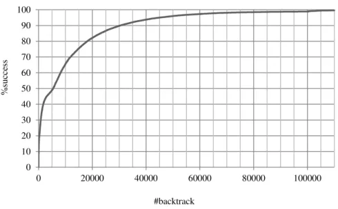
In this thesis, we start by studying the impact of restarts in randomized backtrack search algorithms for solving CSP (Baptista and Azevedo, 2010). For that, we show that the well-known n-queens problem has a heavy-tail distribution (Gomes et al., 2000), and present empirical evidences that restarts can effectively improve the time to solve the n-queens problem. We also implement a conflict-driven variable heuristic and present empirical evidence that this heuristic effectively improves the time to solve the n-queens problem.

Then we focus our work on domain splitting search, where we generalize the work presented in (Lecoutre et al., 2007a) about nogoods recording from restarts. These are nogoods learned from the last branch of the search tree, just before the restart occurs. A backtrack search algorithm, with 2-way branching is used. In (Baptista and Azevedo, 2011) we generalized the learned nogoods but now using domain-splitting branching and set branching. Domain-splitting search splits the branching variable in two parts, which is, in some sense, similar to SAT branching, which expectedly should be better when applying SAT techniques.

1.3

T

M

restart strategy can also have impact in the performance. So, we study different restart strategies associated with a backtrack search algorithm with domain splitting, and information from nogoods in the variable selection heuristic (Baptista and Azevedo, 2012a). Restarting means learning information from nogoods. From the empirical study we conclude that frequent restarts are better, and a linear incremental restart strategy is better than a geometrical one.

The empirical results on using the activity of variables occurring in nogoods have shown the importance of using this information. We have managed to use this information to create two novel heuristics, which incorporate nogoods information in the well known Fail First dom heuristic and in the state of the art conflict directed dom/wdeg

heuristic. The obtained results indicate a promising research direction which integrates the use of restarts, nogoods and heuristics based on nogoods information.

Part of this Thesis work was already published. An initial paper was presented in the Doctoral program of CP’10, introducing the main idea of this Thesis (Baptista and Azevedo, 2010). A paper in the Proceedings of the 15th Portuguese Conference on Artificial Intelligence, published by Springer, focuses on the generalization of nogood recording from restarts in domain splitting search (Baptista and Azevedo, 2011). Then, two other papers, with initial results on restarts, nogood recording from restarts in domain splitting search, and heuristics using nogoods information, were accepted in two workshops of the main conferences of this Thesis area, SAT’12 (Baptista and Azevedo, 2012a) and CP’12 (Baptista and Azevedo, 2012b).

1.3

T

M

We start by an overview of constraint solving, where we cover Constraint Satisfaction Problem and Satisfiability Problem. We define the two problems and explain the techniques used for solving those problems. For the Constraint Satisfaction Problem we present and explain the problems used in this thesis.

through the central fail-first principle and focusing on the state of the art dom/wdeg

heuristic. Then we approach SAT heuristics with a special attention to the widely used

vsids heuristic. In the restarts chapter we start by the use of randomization and the very

important heavy-tail phenomena. Then we approach restarts strategies and the learning of nogoods from restarts. At the end of the chapter we present the results of using restarts on our tested problem instances.

The next two chapters are the main contributions of this thesis. The first one is a theoretical contribution where we present a generalization of learning nogoods from restarts, but now in the context of domain splitting search, which we call ds-nogoods. These ds-nogoods alone prove not to be relevant in pruning the search space. But, in the following chapter we present a novel technique (inspired in SAT) of successfully using information from ds-nogoods, recorded from restarts, in the heuristic decisions.

2

C

ONSTRAINT

S

OLVING

Constraint solving is a technique from the area of Artificial Intelligence related with problem solving. It allows us to define a problem and constraints that must be satisfied. The problem is defined by means of variables and the constraints by means of relations among variables. Then the computer, using a problem solving algorithm, solves the problem and presents the solution. The problem solving algorithm is a search algorithm and a solution is a valuation for the variables defining the problem.

In the limit, using constraint solving would not require programming the solution. The user would state the problem and constraints in a declarative form, and the artificial intelligence agent will use a problem solving algorithm to find a solution.

2.1

C

S

P

2.1.1 Definitions

A Constraint Satisfaction Problem (CSP) consists of a set of variables, each with a domain of values, and a set of constraints on a subset of these variables.

associated to them, where Di (i∈ 1…n) is the set of possible values for variable xi. So, each variable xi ranges over the domain Di, not empty, of possible values. An assignment

xi = vk, where vk ∈ Di, corresponds to instantiating variable xi with value vk from its domain Di. Now consider a set of constraints C={C1,…,Cm} over variables of X. Each constraint Cj (j∈ 1…m) involves a subset Xj⊆X, stating the possible value combinations of the variables in Xj. If the cardinality of Xj is 1 we say that the constraint is unary, and if the cardinality is 2 we say that the constraint is binary. We can see a constraint as a restriction on the allowed values (of domain) for a set of variables. Hence, a CSP is a triple, (X,D,C), consisting of a set X of variables with respective domains D, together with

a set C of constraints.

We must define for the CSP what a solution is. A problem state is defined as the assignments of values to some (or all) variables, among the respective domains. An assignment is said to be complete if every variable of the problem has a value (is instantiated). An assignment that satisfies all constraints (does not violate constraints) is said to be consistent, otherwise it is said to be inconsistent. So, a complete and consistent assignment is a solution to the CSP. A problem is satisfiable if at least one solution exists. More formally, a problem is satisfiable if there exists at least one element from the set

D1×…×Dn which is a consistent assignment. A problem is unsatisfiable if it does not have solution. Formally, in this case, all elements from the set D1×…×Dn are inconsistent assignments.

In this thesis we are interested in constraint satisfaction problems that use domains with finite number of elements. We call these, CSPs with finite domains (CP(FD)).

To illustrate a CSP problem, let us consider a simple problem P=(X,D,C), defined as

following,

X = {x1, x2, x3, x4}

D = {{1, 2, 3}, {1, 2, 3}, {1, 2, 3}, {1, 2, 3}}

C = {x1 ≠ x2, x2 ≠ x4, x2 ≠ x3, x3 ≠ x4}

And the partial assignment

2.1

C

S

P

In this case, because constraint x1 ≠ x2 is violated, the partial assignment is not consistent. This means that this assignment could not be part of a solution to problem P.

Consider again problem P, but now the following complete assignment

{x1 = 1, x2 = 3, x3 = 1, x4 = 2}

As it is easily seen, this is a consistent assignment, since it does not violate any constraint. And because it is complete, it is a solution to problem P.

In the example, we use the binary constraint not equal to. There is no list of possible

constraints, since it depends on the specific solver implementation that is used. Nevertheless, the most common constraints that are expected to be implemented are arithmetic operators (+, -, *, /, …), mathematical operators (sqr, sqrt, pow, min, max, …),

logical operators (AND, OR, …) and relation operators (equal to, not equal to, inequalities).

All these constraints are unary or binary, but, a very important type of constraints, known as global constraints, plays an important role in modelling CSP. These global constraints allow a better modelling of a problem. One global constraint can include more than two variables, and, in the limit, include all the variables in the problem. The use of global constraints could simplify the modelling, since, typically, one global constraint replaces various binary constraints. One example is the very important alldifferent

(Hoeve, 2001) global constraint. This constraint guarantees that all variables must have different values. The alldifferent constraint replaces all the pairwise variables with the

binary not equal to (≠) constraint. In general, the use of global constraints are also more

efficient than the use of all the equivalent binary constraints.

2.1.2 Search algorithms

may be effective at finding a solution if one exists. Local search is an example of an incomplete algorithm. In this thesis we will use a complete backtrack search algorithm.

A backtrack search algorithm performs a depth-first search. At each node an uninstantiated variable is selected based on a variable selection heuristic. The branches out of the node correspond to instantiating the variable with a possible value (or constraining to a set of values) from the domain, based on a value selection heuristic. The constraints ensure that the assignments are consistent.

At each node of the search tree, an important look-ahead technique, known as constraint propagation, is used to improve efficiency by maintaining local consistency. This technique can remove, during the search, inconsistent values from the domains of the variables and therefore prune the search tree. A widely used look-ahead technique is MAC (Sabin and Freuder, 1994), it maintains during the search a property known as Arc Consistency. This property guarantees that in a binary constraint, the values in the domain of one of the variables have support in the values of the other variable. The notion of support means that one value is possible in the variable domain if exists other values (at least one) on the other variable domain for which the constraint is not violated. This is checked for all the values in the domains of the two variables of the binary constraint. The values that do not have support can be safely removed. This property is implemented by means of a propagator associated to each constraint. Every time the domain of a variable changes, propagators for constraints over that variable are applied. This is also known as filtering. Constraints that use more than two variables, e.g., global constraints, implement their own propagators. This extension of Arc Consistency to non-binary constraints is known as Generalized Arc Consistency (GAC).

2.1

C

S

P

2.1.3 Branching schemes

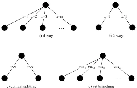
At each node of the search tree, different branching schemes could be used. In Fig. 2.1

we can see graphically the four different branching schemes. Two traditional and widely used branching schemes are the d-way and 2-way. In the first one, at each node, branches are created, one branch for each of the possible values of the domain of the variable associated with the node. Branches correspond to assignments of values to variables. In the 2-way branching scheme two branches are created out of each node. In this scheme a value vk is selected from the domain Dk of a variable xk, associated with the node. The left branch corresponds to the assignment of the value to the variable, and the right branch is the refutation of that value. This can be viewed as adding the constraint xk=vk to the problem, in the left branch; or, if this fails, adding the constraint xk≠vk to the problem, in the right branch. An important difference in these two schemes is that in d-way branching the algorithm has to branch again on the same variables until the values of the domain are exhausted. In 2-way branching, when a value assignment fails, the algorithm can choose to branch on any other unassigned variable.

x≤5 x>5

x=1 x≠1

x=1 x=2 x=3 x=m

. . .

x=s1 x=s2 x=s3 x=sm

. . .

a) d-way b) 2-way

c) domain splitting d) set branching

Fig. 2.1. Example of different branching schemes

Set Branching refers to any branching scheme that splits the domain values in different sets, based on some similarity criterion (Balafoutis et al., 2010). The algorithm then branches on those sets. In each branch, the search algorithm constrains the variable to the values in the corresponding set. Note that 2-way and domain splitting branching schemes can be viewed as a particular case of set branching. And also d-way branching is a particular case of set branching, where a set is constructed with each value of the domain of the variable.

2.1.4 Learning

Learning in the context of artificial intelligence tries to adapt the agent (implementing some algorithm) to new situations. Information gathered from the world could be used to improve the future action of the agent. As the agent observes the world and makes decision to interact with the world, learning could occur. Learning can be a simple memorization of some situation, the detection and extrapolation of patterns, or the creation of a more complex logical structure, e.g., an entire scientific theory (Russell and Norvig, 2002).

2.1

C

S

P

observation of the conflict situation and the nogood is created to explain the conflict. These nogoods can be viewed as a safeguard of the conflict, ensuring that the conflict does not occur again in the future.

Nogood recording was introduced in (Dechter, 1990), where a nogood is recorded when a conflict occurs during a backtrack search algorithm. Those recorded nogoods were used to avoid exploration of useless parts of the search tree.

Standard nogoods correspond to variable assignments, but more recently, a generalization of standard nogoods, that also uses value refutations, has been proposed by (Katsirelos and Bacchus, 2003, 2005). They show that this generalized nogood allows learning more useful nogoods from global constraints. This is an important point since state of the art CSP solvers rely on heavy propagators for global constraints. The use of generalized nogoods significantly improves the runtime of CSP algorithms. It is also important to notice that these generalized nogoods are very much like clause recording in SAT solvers.

Recently, the use of standard nogoods and restarts in the context of CSP algorithms was studied (Lecoutre et al., 2007a, 2007b). They record a set of nogoods after each restart (at the end of each run). Those nogoods, named nld-nogoods, are computed from the last branch of the search tree. So, the already visited tree is guaranteed not to be visited again. This approach is similar to one already used for SAT, where clauses are recorded, from the last branch of the search tree before the restart (search signature) (Baptista et al., 2001). Recorded nogoods are considered as a unique global constraint with an efficient propagator. This propagator uses the 2-literal watching technique introduced for SAT (Moskewicz et al., 2001). Experimental results show the effectiveness of this approach. More recently (Jimmy H. M. Lee et al., 2016) show that nld-nogoods, in a reduction version, are increasing. And (Glorian et al., 2017) propose different ways to reason with those increasing nogoods.

of CP(FD) and SAT. They conclude that the combination of CP(FD) search with learning can be extremely powerful.

Learning general constraints, proposed in (Veksler and Strichman, 2015, 2016), is a stronger form of learning which, instead of learning generalized nogoods, learns constraints. This new learning scheme is inspired on conflict analysis of SAT solvers. It traverses a conflict graph backwards for constructing a conflict constraint. Inference rules for different types of constraints are used for the construction of the learned constraint. Still, as the authors explain, this is an initial work and needs further developments of new inference rules for other types of constraints. They present promising results of this learning scheme, which is implemented for some constraints in the state of the art Haifa CSP solver (Veksler and Strichman, n.d.). This CP(FD) Solver uses techniques from SAT, namely, a variable selection heuristic similar to vsids (Moskewicz et al., 2001), a

phase saving mechanism (Pipatsrisawat and Darwiche, 2007), restarts and learning. It is somehow related with our work, since it uses restarts, learning (a different scheme) and heuristics based on learning.

2.1.5 Examples of CSP Problems

In this section we will present some CSP problems and show how they could be modeled. The presented problems are the ones that we will use in our empirical study. So, besides explaining the problems we also present and explain how the problems are modeled using the Comet System.

The Comet system was the solver that we used in this thesis to implement and test our proposed solutions. So, we will use this section for presenting and explaining how we model the used problems in Comet. We will use the first problem to explain some relevant parts of the Comet language.

2.1.5.1 N-Queens

The n-queens problem is the problem of putting n queens in an n by n matrix,

2.1

C

S

P

problem of size n, i.e., putting 4 queens in an n by n chessboard. The fist example, a)

solution, represents a solution for the problem, since all the queens are in a cell they do

not attack each other. In the second example, b) conflict, the two queens in the third and

fourth column are attaching each other in the diagonal, which configures a conflict situation. Hence, this second example is not a solution for the problem.

♛

♛

♛

♛

♛

♛

♛

♛

a) solution b) conflict

Fig. 2.2. Example of n-queens problem

To model the n-queens problem we use one variable for each column. Hence, the variables x1, …, xn, represent the columns of the chessboard. Each column can only have one queen, so, each variable contains the number of the row where the queen is. Thus, the domain of each variable is the possible rows, i.e., the set {1, …, n}.

For implementing the chess rule of non-attacking queens we must create constraints specifying that, for each queen, there are no more queens in the same row, nor in the same diagonal. For the first case we must guarantee that variables of the problem have different values, i.e., have different rows. We could define a constraint, for each pair of variables, specifying that each variable in the pair are different,

xi≠ xj, where 1 ≤ i,j ≤ n and i < j

xi – i ≠ xj – j, where 1 ≤ i,j ≤ n and i < j

xi + i ≠ xj + j, where 1 ≤ i,j ≤ n and i < j

Of course, in practical terms, if the solver allows global constraints, it is better to use them. For this problem, instead of using the binary constraints for all the pairs we use only alldifferent global constraints. So, we end up with the following three constraints,

alldifferent(x1, x2, …, xn)

alldifferent(x1 – 1, x2 – 2, …, xn – n)

alldifferent(x1 + 1, x2 + 2, …, xn + n)

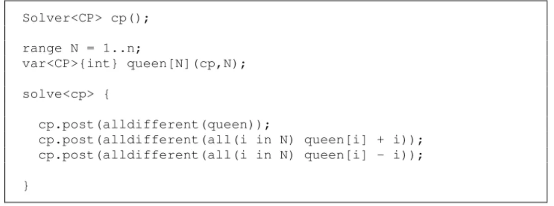
The code for the Comet model of the n-queens problem is shown in Fig. 2.3. We only

show relevant parts of the modelling code. In Comet, we first need to create a CP solver, which will contain all the relevant parts of the solver, namely, the variables, the domains and the constraints. To be more precise, the constraints are posted in the solver only in the

solve<cp> body, which is related with the search algorithm.

Solver<CP> cp();

range N = 1..n;

var<CP>{int} queen[N](cp,N);

solve<cp> {

cp.post(alldifferent(queen));

cp.post(alldifferent(all(i in N) queen[i] + i)); cp.post(alldifferent(all(i in N) queen[i] - i));

}

Fig. 2.3. Comet model for N-Queens

So, the first line of the code defines the CP solver and the next two lines are related with the variables. A range of values is defined, which is used as the domain of the variables. For the variables for the queens we use an array of Integers whose domains are the defined range of values. Then, the three constraints are posted in the solver variable, inside the solver<cp> body. In this case we use the alldifferent global constraint, as

already explained. The first alldifferent constraint receives the array of queens, which

2.1

C

S

P

do not have arrays, but Comet language allows the creation of arrays on the fly. This is what is done in the last two posts, an array is created with variables having the difference, in one case, and the sum, in the other case. Then, the alldifferent constraint guarantees, in

each case, that variables must be different.

2.1.5.2 Magic square and Talisman Square

A magic square of size n is an n by n matrix with all the numbers from 1 to n2_{, such that} the sum of each row, column and the two main diagonals are equal to a known magic constant. This is problem number 19 from CSPLIB (Walsh, n.d.). The magic constant is computed as

1

2 + 1

An example of a magic square can be seen in Fig. 2.4. Because it is a 4 by 4 square,

all the cells have different numbers from 1 to 16. The magic square, in this case, is 34 and can be easily checked that it corresponds to the sum of the number in each column, rows and the two main diagonals.

16 3 2 13

5

9

4

10 11 8

6 7 12

15 14 1

Fig. 2.4. Example of a Magic Square

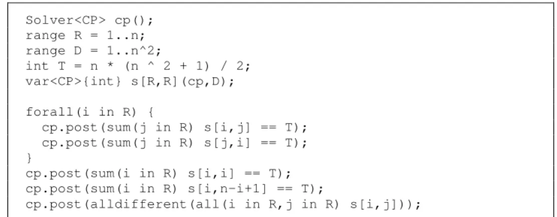
The Comet model for the Magic square is presented in Fig. 2.5 (note that, for

simplicity we eliminate the solve(cp) scope). To model the magic square we need n2

variables, one for every position of the matrix, hence we use a two-dimensional array for the variables. The domain of those variables are all the possible numbers, i.e., the set {1, …, n2_{}. We need to add constraints for the sums of all the n rows, n columns, and the two} diagonal main diagonal. Finally, an alldifferent constraint is used for all the variables, so

Solver<CP> cp(); range R = 1..n; range D = 1..n^2;

int T = n * (n ^ 2 + 1) / 2; var<CP>{int} s[R,R](cp,D);

forall(i in R) {

cp.post(sum(j in R) s[i,j] == T); cp.post(sum(j in R) s[j,i] == T); }

cp.post(sum(i in R) s[i,i] == T); cp.post(sum(i in R) s[i,n-i+1] == T);

cp.post(alldifferent(all(i in R,j in R) s[i,j]));

Fig. 2.5. Comet model for Magic square

A Talisman square of size n is a magic square of size n but with constraints stating

that the difference between any two adjacent cells (including diagonal adjacent cells) must be ‘greater than’ some constant, k. So, to the Magic square Comet model we

include, for each cell, constraints guaranteeing that the difference with adjacent cells is greater than k (Fig. 2.6). Note that for each cell we only need to add 4 constraints, for 4

directions that are not symmetric between then. In this case we consider the directions, by the order they appear in the Comet model, South, South-East, East and North-East. The

constraints related with the other symmetric directions are considered when those cells were processed. Adding constraints to the 8 adjacent cells would repeat constraints.

forall(i in R,j in R) { int v; int h;

v=1; h=0;

if ((i+v >= 1 && i+v <= n) && (j+h >= 1 && j+h <= n)) cp.post(abs(s[i,j]-s[i+v,j+h])>k);

v=1; h=1;

if ((i+v >= 1 && i+v <= n) && (j+h >= 1 && j+h <= n)) cp.post(abs(s[i,j]-s[i+v,j+h])>k);

v=0; h=1;

if ((i+v >= 1 && i+v <= n) && (j+h >= 1 && j+h <= n)) cp.post(abs(s[i,j]-s[i+v,j+h])>k);

v=-1; h=1;

if ((i+v >= 1 && i+v <= n) && (j+h >= 1 && j+h <= n)) cp.post(abs(s[i,j]-s[i+v,j+h])>k);

}

Fig. 2.6. Extra constraints for the Talisman square Comet model

2.1

C

S

P

we remove from the Talisman square the constraints related with the sum of the magic constant. Of course, the constraint guaranteeing that all the variables of the matrix are different is maintained.

2.1.5.3 Latin squares

A Latin square of size n is an n by n matrix, such that each row and column has the

numbers 1 to n without repetition. This is described in problem number 3 of the CSPLIB

(Pesant, n.d.).

3 1 2 4

4

1

2

2 3 1

3 4 2

4 1 3

3

2

4

4 2

1

a) filled b) partially filled

Fig. 2.7. Example of Latin squares

In Fig. 2.7 we can see two examples of Latin squares of size 4. The first one is fully

filled with the numbers 1 to 4 in each row and column, without repetition. The second one is partial filled, maintaining, for the already filled numbers, the same constraints in each row and column.

Solver<CP> cp(); range R = 1..n; range D = 0..n-1;

var<CP>{int} s[R,R](cp,D);

forall(i in R) {

cp.post(alldifferent(all(j in R) s[i,j])); cp.post(alldifferent(all(j in R) s[j,i])); }

Fig. 2.8. Comet model for Latin square

The Comet model for this problem is presented in Fig. 2.8. It has n2 variables, one for

every position of the matrix, whose domain is the set {1, …, n}. For each column and row

We also use a variation of this problem, called Quasigroup With Holes (QWH), which is a partial filled Latin square where some cells have a pre-defined number. This problem is known to be more difficult than the Latin squares.

The well-known Sudoku problem is a Latin square with additional alldifferent

constraints for the interior squares. A widely used Sudoku puzzle is a Latin square of size 9 with pre-defined numbers, and with nine interior squares of 3 by 3 where the numbers 1 to n must also occur without repetition. The Sudoku problems can be generalized to other

sizes, provided that the size is a perfect square, which guarantee the existence of the interior squares.

2.1.5.4 Golfers

This is known as Social Golfers Problem and is also included in CSPLIB as problem number 10 (Harvey, n.d.). The objective of this problem is scheduling g groups of s

golfers over w weeks, such that golfers do not repeat partners.

Solver<CP> cp();

range Groups = 1..gc.groups; range Slots = 1..gc.slots; range Weeks = 1..gc.weeks;

range Golfers = 1..(gc.groups * gc.slots);

var<CP>{int} golfer[Weeks,Groups,Slots](cp,Golfers);

forall (w in Weeks)

cp.post(alldifferent(all(g in Groups, s in Slots) golfer[w,g,s]));

forall (w in Weeks) forall (g in Groups)

forall (ws in Weeks : ws > w) forall (gs in Groups)

cp.post(sum(s in Slots, t in Slots)

(golfer[w,g,s]==golfer[ws,gs,t])<=1);

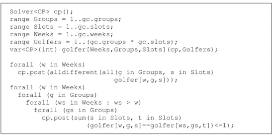
Fig. 2.9. Comet Model for Golfers (without symmetries)

The Comet model for this problem is presented in Fig. 2.9. We define ranges for the

2.1

C

S

P

The first set of constraints is used to ensure that all the golfers play in each week. It is an alldifferent constraint for each week, stating that all the variables in that week is

different, so, golfers only play once in each week. The second set of constraints is used to define that golfers do not repeat partners in different weeks.

This problem is known to have different symmetries. We do not present here constraints for symmetry breaking, but we use constraints for breaking the most important symmetries. Namely, we consider the following symmetries: players inside groups can be exchanged; groups inside weeks can be exchanged; weeks can be exchanged; and players can be renumbered.

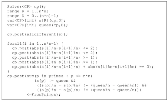
2.1.5.5 Prime Queen

This problem is known as Prime queen attacking problem and is CSPLIB problem number 29 (Bessiere, n.d.). This problem uses a chess board of size n by n, whose cells

must be numbered from 1 to n2, without repetitions. Any number i + 1 must be reached by

a knight move from the cell containing number i. Also, a queen must be put in a cell such

that the number of free primes is minimal (primes that are not attacked by the queen).

Solver<CP> cp(); range R = 1..n*n; range D = 0..(n*n)-1; var<CP>{int} s[R](cp,D); var<CP>{int} queen(cp,D);

cp.post(alldifferent(s));

forall(i in 1..n*n-1) {

cp.post(abs(s[i]/n-s[i+1]/n) <= 2); cp.post(abs(s[i]%n-s[i+1]%n) <= 2); cp.post(abs(s[i]/n-s[i+1]/n) >= 1); cp.post(abs(s[i]%n-s[i+1]%n) >= 1);

cp.post(abs(s[i]/n-s[i+1]/n) + abs(s[i]%n-s[i+1]%n) == 3); }

cp.post(sum(p in primes : p <= n*n) (s[p] != queen &&

((s[p]/n - s[p]%n) != (queen/n - queen%n)) && ((s[p]%n - s[p]/n) != (queen%n - queen/n))) <=FreePrimes);

Fig. 2.10. Comet model for Prime queen

The Comet model used for this problem is presented in Fig. 2.10. We use an array of

position on the chessboard (the numbers from 0 to n2–1). We also need a variable for the

position of the queen. The first constraint is an alldifferent guaranteeing that all the

numbers are in different positions. Then, for each successive numbers (successive position in the array of variables), we define a set of constraints which guarantee the knight move.

This problem is formulated as an optimization problem, since it tries to minimize the total number of free primes. Because our work is concerned with satisfaction problems we transform this problem in a satisfaction problem. So, we add a constraint stating that the number of free primes must be less than or equal than some constant. In this way it is possible to solve various decision problems, each time with a smaller number of free primes. The prime numbers are pre-computed and saved in the primes array.

2.1.5.6 Cattle Nutrition

This is a real world problem related with finding the best combination of Cattle food, considering the nutritional requirements of Cattle. This problem is typically from the Linear Programming area, but we have used a discrete representation of the continuous variables of the problem, for use in the CP(FD) model.

Solver<CP> cp();

range D = 0..(maxGramas/gran)+1;

var<CP>{int} vars[R](cp,D); //one entry for each food

cp.post(sum(i in R)(vars[i]*(gran/1000.0)*infoAlimentos[i].ca) <= necessidades.ca * (1+necessidades.eMax));

cp.post(sum(i in R)(vars[i]*(gran/1000.0)*infoAlimentos[i].ca) >= necessidades.ca * (1-necessidades.eMin));

Fig. 2.11. Partial Comet model for Cattle Nutrition

For this problem, a set of different Cattle food is considered. Then, the purpose is to define the amount of each type of food, such that a set of nutritional requirements constraints are satisfied. We present in Fig. 2.11 a partial Comet model for this problem.

First, we define the discrete representation for the amount of food with a defined granularity, gran. Then we use one array of variables with one position for each type of

2.2

S

P

different Cattle food with nutrition information, which is used to select the nutrition information of the used Cattle food and saved in the array infoAlimentos.

For each type of nutrition requirements we have two constraints, stating that the food amount must be within a minimum and maximum value. In Fig. 2.11 we see an example

of such a constraint for the calcium requirements.

2.2

S

P

2.2.1 Definition

A propositional satisfiability problem (SAT) is a particular case of a CSP where the variables are Boolean, and the constraints are defined by propositional logic expressed in conjunctive normal form. In spite of this relation, SAT is a well-known decision problem, used for modeling combinatorial problems, and for which a full line of completely independent research is in continuous growth. In any case, SAT and CSP share many techniques and have benefited from each other developments (Bordeaux et al., 2006).

SAT was the first decision problem proved to be NP-Complete (Cook, 1971). It has many applications to real world problems, since SAT algorithms have proved to be very successful on handling large search spaces, due, primarily, to the ability of exploiting problem structure (Marques-Silva, 2008).

Considering a propositional logic formula, the propositional satisfiability problem is a decision problem trying to satisfy the formula using assignments to the variables of the formula. More formally, consider the Boolean variables xi, i=1, …,n, of the propositional logic formula; SAT can be defined by finding an assignment to all the Boolean variables

xi in the formula, such that the formula becomes a logical truth, i.e., satisfiable. Instead of using propositional formulas expressed in the full syntax of propositional logic, SAT uses, without loss of generality, formulas expressed in conjunctive normal form (CNF). A CNF formula φ is a conjunction of clauses wi, i=1,…,m, where each clause is a disjunction of literals. A literal is an occurrence of a Boolean variable xi or its negation

false (or 0 – zero) can be assigned. A variable with no assigned value is said to be a free

variable. Accordingly, a literal can have a Boolean value or be a free literal. A clause (wi) is said to be satisfied (wi=1) if at least one of its literals has the value true, unsatisfied (wi=0) if all of its literals have the value false and unresolved otherwise (i.e., when it is not possible to know the value of the clause). This last case occurs if none of the literals have the value true, but some, and not all, have the value false. An unresolved clause with

only one free literal is said to be a unit clause. This type of clause plays an important role in the search space reduction of the search algorithm, as it will be explained in the next section. A CNF formula is said to be satisfied, φ = 1, if all its clauses are satisfied,

unsatisfied, φ = 0, if at least one of the clauses is unsatisfied. Otherwise, the formula is

unresolved, i.e., there are no unsatisfied clauses and at least one of the clauses is unresolved.

To illustrate a SAT problem, let us consider the CNF formula, which has three clauses,

φ=(x1˅ x2) ˄ (x1˅¬x3˅¬x2) ˄ (x3˅¬x2). And the set of assignments

{ x1 = 0, x3 = 1}

Considering these assignments we rewrite the CNF formula φ with the Boolean values instead of the variables

φ=(0˅ x2) ˄ (0˅0˅¬x2) ˄ (1˅¬x2).

So, those assignments make the first and second clause unresolved. In this case, these two clauses are unit clauses, because all the literals, except one, have the value false. The

third clause is satisfied because one of the literals, x3, is true. Hence, the formula is unresolved, because there are no unsatisfied clauses, some clauses (one in this case) are satisfied and other clauses are unresolved, which per se does not allow us to know the

state of the formula.

For another example, consider again the same CNF formula φ and the set of assignments

2.2

S

P

Considering now these assignments we rewrite the CNF formula φ with the Boolean values instead of the variables

φ=(1 ˅ x2) ˄ (1 ˅ 0 ˅¬x2) ˄ (1 ˅¬x2).

In this case all the clauses are satisfied because all the clauses have one literal with value true and, hence, the formula is satisfied.

2.2.2 Search Algorithms

As already referred the propositional satisfiability problem belongs to the well-known NP-Complete class of problems. Algorithms for this class of problems have exponential time complexity in the worst case, unless P = NP. The principal approach for solving

SAT is based on the Davis, Putnam, Logemann and Loveland (DPLL) procedure (Davis et al., 1962; Davis and Putnam, 1960), which is basically a backtrack search algorithm which implicitly searches a binary tree of decisions, defined by the 2n _possible assignments of the Boolean variables, where n is the number of variables in the problem.

In each node of the search tree a free Boolean variable is selected for branching. Out of each node, two branches are created: one for the decision of assigning true; and the

other for the decision of assigning false to the selected variable. The selection of the

variable is typically based on heuristic selection, being vsids (variable state independent

decaying sum) the most widely used variable selection heuristic (Moskewicz et al., 2001) and considered state-of-the-art. The order by which the two Boolean values are tested may also depend on heuristics.

After each decision, some of the clauses could become unit clauses, which allows a technique known as unit propagation (Davis and Putnam, 1960) to be applied. This technique identifies necessary assignment for variables. A unit clause has only one free literal (and all the others are false), so, to become satisfied it is necessary that the free

literal becomes true. Note that after implying the necessary Boolean value to a literal, and

BCP reduces the search space, pruning branches of the search tree corresponding to the implied variables.

The search tree maintains a partial solution to the problem, consisting of assignments of Boolean values to the variables. When a node is reached where all the clauses become satisfied, the search ends with a solution. But, if during the search a node is reached where, at least, one unsatisfied clause exists, the search can no longer continue and the search must backtrack to try other value combinations. The search backtracks to the most recent node where only one of the two Boolean values has been tried. This form of backtracking is known as chronological backtracking. If the search space is exhausted without reaching the situation where all the clauses are satisfied, the problem has no solution because the formula is unsatisfiable.

Other more interesting form of backtracking is non-chronological backtracking. Instead of backtracking for the most recent node, it is able to backtrack to a node identified as one of the causes of the conflict. This form of backtracking is used in state-of-the-art SAT solvers and has the advantage of skipping irrelevant decisions for the failure, which, in practice, corresponds to pruning irrelevant search tree branches. An important form of non-chronological backtracking is known as Conflict-Directed Backjumping and was introduced by (Prosser, 1993). Nevertheless, current SAT solvers use a form of non-chronological backtracking that is associated with another very important technique known as clause learning from conflicts.

2.2

S

P

When a conflict occurs, the CDCL algorithm identifies its causes. For this, the algorithm maintains an implication graph created with the implied assignments, which were made by the Boolean Constraint Propagation mechanism. The CDCL algorithm identifies the conditions, by means of the set of assignments, which originate the conflict. A new clause, that explains the conflict, is then created and recorded. This recorded clause is known as conflict clause, or nogood, and is used by the CDCL algorithm in the remainder of the search tree as part of the CNF formula. This conflict clause is a safeguard, guaranteeing that the assignments that drive the search to a conflict do not to happen again, hence, pruning the subsequent search tree.

Conflict clauses are recorded every time a conflict occurs. This could lead the algorithm to run out of memory. Note that, in the worst case, the number of conflicts is exponential in the number of variables, so, recording all the conflict clauses could be impossible in practice. On the other hand, large conflict clauses are known to be of little importance for pruning the search tree (Silva and Sakallah, 1996). So, in practice, SAT solvers define conditions for deleting those larger conflict clauses.

The use of restarts is an important improvement on CDCL solvers (Baptista and Silva, 2000), and is, currently, widely used. It continuously runs the search algorithm, from the beginning, giving, on each run, a new opportunity for solving the problem. Typically, the restart occurs when a cutoff value is reached; the search stops and then starts again a new run. To guarantee algorithm completeness, the cutoff value is incremented after each restart. Note that, because of clause recording of CDCL solvers, after each restart the search no longer starts from scratch, it starts with learned clauses retained from past runs.

the search backtracks. The latter improvement uses the occurrence of variables in conflict clauses, and also, from time to time, the occurrences of variables are divided by a constant. This is a very low overhead variable selection heuristic that prefers variables participating in recent conflicts and is known as variable state independent decaying sum (vsids).

Due to non-chronological backtracking and restarts, trashing of good decisions can occur, requiring the search to redo that same search space in the future. To avoid this loss of decisions, a mechanism of decision caching can be used that makes the same decision when the variable is selected. This was introduced in (Pipatsrisawat and Darwiche, 2007), and is known as phase-saving, which is typically associated with rapid restarts.

2.3

S

F

R

Constraint Satisfaction Problems and Satisfiability Problems represent very important areas of research within the broader area of Artificial Intelligence. They both are decision problems and share many techniques. Still, they have independent research directions which have resulted in different approaches in each area. In the context of our research interest we highlight the widely use of restarts and learning in SAT algorithms compared with the only emerging use in CP(FD) algorithms.

3

H

EURISTICS

As already discussed, backtrack search algorithms are widely used for solving constraint satisfaction problems. A key element of these algorithms is the order in which variables are selected for branching. Also, but not so important, is the order in which the values for the selected variable are tested. As it is widely known, a bad decision on the next variable to select could drive the search for unpromising regions of the search space. This results in combinatorial explosions of the search space.

Near the root of the search tree, a bad decision has more impact, because a bigger tree exists under that bad decision, and, consequently, a bigger search space explosion exists. This is why good heuristic decisions are important near the root of the search tree. Unfortunately, that is not always the case since, typically, at the beginning of search, the heuristic is not well informed.

An adaptive heuristic can gather information from the already explored search space. With that information we can tune the heuristic to become more informed. We still have the problem of bad first decisions, occurring near the root of the search tree. But as the search evolves, the problem of bad decisions near the root tends to fade away, due to more informed decisions.

making more informed decisions. We can see the impact of this when results are discussed.

It is also important to notice that, in this thesis, we are not interested in problem dependent heuristics. Our focus is on general purpose heuristics, that are independent of the domain of the problem considered.

The remainder of this chapter is organized as follows. We start by comparing static versus dynamic variable ordering heuristics. Then we focus on the important fail first principle. Next we focus on weighted based heuristics and then we explain more recent heuristic strategies. Finally we overview the more important SAT heuristics, namely the one based on conflicts, as this is central in this thesis.

3.1

S

Static variable ordering (SVO) heuristics only use information from the structure of the initial problem, without using information from the ongoing search. The order for selecting the branching variables is defined before the search and is fixed during the search (this is why they are also called fixed variable ordering). This means that, at each node of the search tree, the algorithm selects for branching the next free variable based on the predefined ordering of the variables.

On the other hand, dynamic variable ordering (DVO) heuristics are branching variable selection heuristic strategies that use information of the ongoing search to change the ordering of the variables. Hence, at each node of the search tree, the algorithm selects for branching the next free variable based on the current CSP at that point, which is dependent on the (partial) assignment already made. This means that at each node a different ordering can exist.

The most basic SVO heuristic selects the next branching variable based on the lexicographical order (lex). So, by simply changing the names of the variables in the

3.2

T

common situation, when different variables have the same heuristic value. Faced with that situation, the backtrack search algorithm must break ties and chose only one of them. Another widely used heuristic for breaking ties is the random ordering (rand), applied at

each branching node. This heuristic selects randomly among the variables with the best value. As will be explained later, this heuristic is central for restarts. Also notice that the

rand heuristic can also be used by itself. In this case, and due to the void of information

within this heuristic, the backtrack search algorithm will perform a random search. Another SVO heuristic, width, selects the next branching variable based on the

minimum width of the constraint graph (Freuder, 1982). Also using information from the constraint graph in (Dechter and Meiri, 1989) Dechter and Meiri define a heuristic that selects the next branching variable based on the maximum initial degree of the variables,

deg. This heuristic favors variables that are constrained with more of the other variables.

SVO heuristics suffer from an important weakness: they only use information from the initial problem and that may not be enough to solve the problem. DVO heuristics try to solve this question, since information is collected during the ongoing search, and so, the heuristic is modified as the search evolves.

3.2

T

Tring where it is most likely to fail and pruning the search space as soon as possible are two important strategies that help tree searching for CSP (Haralick and Elliott, 1980). It was also shown empirically that changing dynamically the variable search order, based on the actual size of variable domains, has performance improvements, particularly when forward checking is employed.

The fail first (FF) principle, applied to the variable selection heuristic, states that the variable that is most likely to drive the search algorithm to a failure must be selected for branching. The DVO heuristic based on the FF principle states that the next unbound variable to select for branching is the one with the fewest possible values in the domain (the minimum size of the domain), we call this heuristic dom. So, in this context,