District heating systems: the effect of building model complexity on heat demand prediction

(1)

UNIVERSIDADE DE LISBOA

FACULDADE DE CIÊNCIAS

DEPARTAMENTO DE ENGENHARIA GEOGRÁFICA, GEOFÍSICA E ENERGIA

District Heating Systems: the effect of building model complexity

on heat demand prediction

Luís Ferreira Carvalho

Mestrado Integrado em Engenharia da Energia e Ambiente

Dissertação Orientada por:

Guilherme Carrilho da Graça

(2)

(3)

Resumo

As tendências recentes da distribuição populacional indicam que a grande maioria cidadãos europeus irá habitar em cidades. A elevada densidade energética característica destes aglomerados faz com que a gestão do fornecimento de energia seja, cada vez mais, uma área de grande responsabilidade, tanto ao nível da segurança energética, como da sua sustentabilidade económica e ambiental. Os edifícios são responsáveis por cerca de 40% da energia final consumida na União Europeia, sendo assim um setor com elevado potencial na promoção da eficência energética.

Os sistemas de redes de calor são uma alternativa eficiente para o fornecimento de energia na forma de calor em áreas urbanas. Uma das principais vantagens desta solução, num mercado de calor em expansão, é a possibilidade de utilizar recursos energéticos que de outra maneira seriam desperdiçados ou inutilizáveis à escala de um edificio, com destaque para as energias renováveis. A possibilidade de combinação de várias fontes de energia, confere-lhe também uma elevada flexibilidade energética, tornando-se menos sensível à flutuação dos preços dos combustíveis. As centrais de cogeração, de energia eletrica e térmica, são particularmente interessantes neste tipo de aplicações, conseguindo aproveitar o calor anteriormente desperdiçado, face a uma central elétrica convencional. Para além diso, o efeito de escala e a monitorização contínua destes sistemas permite uma maior eficiência na produção de energia contribuindo assim para redução das emissões de gases de efeito de estufa. Os mais recentes desenvolvimentos nestas redes de calor incluem novas estratégias para uma maior integração de fontes de energia renováveis e melhorias na interação entre produtores e consumidores. Como foco principal está a utilização de fontes de calor e distribuição de baixa temperatura, adaptada à redução do consumo energético ao nível dos edifícios. Em resultado, a complexidade destes sistemas aumenta e a necessidade de metodologias mais detalhadas para análise e desenvolvimento torna-se ainda mais evidente. Para o efeito, o uso de modelos computacionais vem permitir e facilitar este processo mas não existe um programa que seja ao mesmo tempo, fácil de usar, rápido, flexível para simular redes e edifícios detalhadamente. As diferenças entre diferentes modelos ao nível da complexidade dos algoritmos e detalhe das variáveis influencia a qualidade e resolução dos resultados, pelo que o uso de um modelo em detrimento de um outro, pode levar a diferentes conclusões, afectando assim o planeamento de um projeto. Desta forma, a escolha do modelo mais adequado a determinado projeto deve ter em conta o tipo de sistemas que estão envolvidos, as variáveis que vão ser estudadas, os dados possíveis de adquirir e não menos importante, o tempo e recursos disponíveis.

Este estudo centra-se na comparação de diferentes modelos para a previsão das necessidades de aquecimento ao nível dos edifícios. Os modelos criados foram simulados com recurso a dois programas, Dymola, com linguagem Modelica, e EnergyPlus. Modelica é uma linguagem de modelação flexivel, baseada em equações e orientada em objectos que permite a criação de modelos de sistemas complexos de diferentes domínios. A sua estrutura modular permite a fácil partilha e reutilização de modelos. As capacidades de simulação detalhada de edifícios com recurso a esta linguagem tem vindo a ser melhorada com a disponibilização de novas bibliotecas de objectos, mas a sua utilização não se torna tão prática ou direta como noutros programas especificamente desenvolvidos para o efeito, como o EnergyPlus. No entanto, as capacidades de cada programa podem ser complementadas através de co-simulação, onde ambos os programas simulam em simultâneo as necessidades de aquecimento de um edifício, denominando-se de co-simulação: o EnergyPlus encarrega-se do balanço térmico do edifício e as cargas de aquecimento são calculadas no Dymola. Foram criados três modelos com diferentes níveis de detalhe tanto ao nível dos

(4)

algoritmos de cálculo como nos parâmetros de entrada: o modelo A é criado no Dymola com base no método horário simplificado da norma ISO 13790; o modelo B é criado no Dymola com base no modelo Rooms.MixedAir da biblioteca Buildings do Modelica; e o modelo C é criado em EnergyPlus e utilizado em co-simulação com o Dymola.

O caso de estudo considera um pequeno bairro de cinco edifícios adjacentes de diferentes tipologias, com baixo nível de isolamento – cenário referência - , adaptado de um exercício parte do projecto IEA Annex 60. Para um dos edifícios, um bloco de escritórios com 727 m2_{de área útil divididos por}

cinco pisos uniformes, foram definidos três cenários de reabilitação ao nível dos elementos da envolvente, opacos e envidraçados, considerando para o efeito um tipo de constução mais recente. As necessidades de aquecimento do caso referência foram obtidos a partir da simulação de todos os edifícios com o modelo A, e nos três cenários seguintes o edifício alvo foi simulado nos modelos A, B e C. As variáveis em estudo foram a necessidade energética anual [MWh] e a carga de pico [kW] de aquecimento, tendo sido também analisado o perfil destas cargas.

Os resultados obtidos para o bairro no cenário de referência apresentam uma necessidade anual de 256 MWh com um pico 106.5 kW, sendo que o edifício alvo representa cerca de 30% deste consumo, com 110 kWh/m2_{. Como esperado a maior redução da necessidade de aquecimento foi verificada}

para o cenário da renovação total, cerca de -28% ao nível do bairro, resultanto de uma redução do consumo do edifício alvo de 90%, atingindo um mínimo de 9.2 kWh/m2_.

Nos três cenários os modelos apresentaram um boa correlação entre si à excepção do cenário de reabilitação dos envidraçados, com uma diferença de 14.3 pontos percentuais entre o modelo B e C no que diz respeito à redução do consumo anual entre os diferentes modelos. Esta variação de 37 MWh compara-se, em magnitude, a cinco vezes a necessidade energética do edificio de escritórios registado no cenário de total renovação.

Com base na análise dos perfis da carga de aquecimento, concluí-se que a diferença nos resultados obtidos pode ter um impacto mais significativo se mais edifícios fossem alvo de reabilitação, com ainda maior impacto em DHS de pequena escala. A co-simulação entre os dois programas provou ser uma solução viável para otimizar a modelação de sistemas e edifícios, permitindo melhorar o processo e reduzir significativamente o tempo de simulação.

Desenvolvimentos futuros deste trabalho incluem o estudo do impacto de cada modelo num sistema integrado onde sejam implementados modelos de unidade de geração recorrendo a diferentes fontes de energia. Desta forma a dinâmica do perfil do consumo dos edifícios terá maior influência no comportamento do sistema como um todo.

(5)

Abstract

District heating systems (DHS) are an efficient alternative for the heat supply in urban areas. One of the main advantages of this solution, in current expansion on the heat market, is the possibility of using heat resources that would otherwise be wasted on unfeasible in smaller scale. Thus, it contributes to improve the efficiency of urban energy systems and reduce CO2 emissions.

Recent developments of DHS are based in new strategies for a large scale integration of renewable energy sources and improvements in the interaction between demand and supply sides, as smart thermal grids. In result, the complexity of these systems increases, and the need of comprehensive integrated approaches to analyze them is becoming even more evident. The use of computational modeling tools are used for this purpose, but there is no single tool that provides detailed, flexible and rapid prototyping for both buildings and systems. However, time and resources available in the early-design stages usually forces the use of more simplified models to calculate the heating demand, which might lead to different conclusions when compared to more detailed ones.

This study presents a comparison of three different building models developed with Modelica (Dymola) and EnergyPlus, with increasing detail in both calculation algorithms and inputs to estimate the heat demand for space heating. The case study considers three retrofit scenarios, with different levels of thermal insulation, for one building in a small neighborhood. The results obtained across the three models registered a maximum variation of 14% on the annual demand and 9% kW of the peak load for the window retrofit scenario.

Based on the analysis of the heat load profiles, it was concluded that the difference in the results obtained can have a higher impact on the district if more buildings were to be retrofitted, taking even more relevance in small-scale DHS.

(6)

List of Figures

Figure 1. Statistics overview on DH usage and network expansion by country (adapted from [18],

data not available for every country). ... 3

Figure 2. Illustrative comparison between previous district heating schemes and the 4th_generation concept [6]. ... 4

Figure 3. Ilustration of building's heat transfer processes. ... 8

Figure 4. BIM environment (Revit) for building analysis [30]. ... 9

Figure 5. Technical chalenges and outcomes of IEA's Annex 60 [33]. ...10

Figure 6. Analytical, Empirical and Code-to-Code processes. [34] ...11

Figure 7. Case study buildings layout. ...12

Figure 8. One thermal zone five resistance and one capacitance model (5R1C) [39]...14

Figure 9. ISO 13790 thermal network implementation in Dymola [35]. ...15

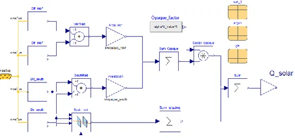
Figure 10. Solar model that calculates the solar gains. ...15

Figure 11. Example of two mixedAir models connection for a multi-zone building (left) encapsulated in the top layer model (right) where weather data and control components are connected to the respective ports. ...16

Figure 12. Office building floor-plan. Geometry input simplification. ...17

Figure 13. Office building geometry ...17

Figure 14. Settings for EnergyPlus export as FMU ...18

Figure 15. Single-zone ideal heat demand control . On the left for model A and B, and on the right for model C. These blocks are replicated for the multi-zone models. ...19

Figure 16. Base Case 600 results from models A, B and C compared with BESTEST range (grey box)...20

Figure 17. District heating demand of the base scenario – Model A. ...22

Figure 18. District heat demand and loads of the three case study scenarios...23

Figure 19. Office building load profiles for each scenario...23

Figure 20. District heat load duration curve for the Window retrofit scenario...24

List of Tables

Table 1. Buildings floor area, Compactness ( Volume/Surface area) and window ratios. ...12

Table 2. Heat transfer coefficient (U-value) and infiltration rates (ACH-air changes per hour) for each scenario...13

Table 3. BESTEST Base Case 600 benchmarking range for heating and cooling demand. ...20

Table 4. Comparison of EnergyP lus nd FMU annual and peak heating demand. ...21

List of Appendices

Table A - 1. Wall construction...29

Table A - 2. Roof construction ...29

(9)

Table A - 4.Window properties - Double pane window ...30

Table A - 5. Building usage and operation inputs ...30

Table B - 1. Exterior wall construction...31

Table B - 2. Roof Construction...31

Table B - 3. Floor Construction ...31

Table B - 4. Internal Wall Construction...31

Table B - 5. Internal floor construction ...32

Table B - 6. Window properties - Wooden window profiles - single glazing ...32

Table B - 7. Window properties - Insulated aluminum profiles –low-e double pane filled with Argon ...33

Table B - 8. Exterior wall construction - retrofit ...33

Table B - 9. Roof Construction - retrofit ...34

Table B - 10. Floor Construction ...34

(10)

Aknowledgements

I would first like to thank professor Jan Hensen for receiving me at the Building Physics and Services research group, Eindhoven University of Technology and for his helpful advice throughout the whole project.

Furthermore, I want to thank Ignacio Torrens for his support and guidance during this research. Also to Luyi Xu and Sanket Puranik for their enthusiasm and availability to help me about the software used.

I want to thank professor Guilherme Carrilho da Graça for supervising the project in my home university and effort made to make this international experience possible.

Special thanks to my mother, Leonor Ferreira, for the constant effort put in my education and for encouraging me to go on Eramus ever since I started my academic journey.

A big thank you to my girlfriend Raquel Barbosa for all her love and patience, especially during my period abroad.

And last but not the least, I also want to thank to all my friends for the support provided during these years, particularly to João Homem and Pedro Silva for the great times in Eindhoven.

(11)

Abbreviations and symbols

ACH Air Changes per Hour

ANSI American National Standards Institute

ASHRAE American Society of Heating, Refrigerating, and Air-Conditioning Engineers

BESTEST Building Energy Simulation Test

BIM Building Information Modeling

BPS Building Performance and Simulation

CHP Combined Heat and Power

DES District Energy Systems

DHS District Heating Systems

EED Energy Efficiency Directive

EPBD Energy Performance of Buildings Directive

EU European Union

FMI Functional Mockup Interface

FMU Functional Mockup Unit

HVAC Heating, Ventilation and Air Conditioning

IDF EnergyPlus Input Files

IEA International Energy Agency

(12)

(13)

District Heating Systems: The effect of building model complexity on heating demand prediction

Chapter 1 - Introduction

Two-thirds of the global primary energy is consumed in cities and by 2050, 84% of the European citizens are expected to live in these high density areas [1]. Buildings represent 36% of CO2 emissions

and 40% of the energy consumption in the EU, with 79% corresponding to space heating and domestic hot water [2]. This means that efforts should be made to improve urban energy systems, reducing the energy demand and greenhouse gas emissions to meet the EU targets by 2050.

In the demand side, higher efficiency targets are being defined to reduce the energy consumption in buildings. The Energy Performance of Buildings Directive (EPBD2010) [3] and Energy Efficiency Directive (EED2012) [4] set minimum performance requirements for new buildings and forces the state members to develop better strategies on energy saving measures and buildings retrofit. From the supply side, district heating systems (DHS) play an important role on the transition to a more sustainable energy system as one of the least-cost and most-efficient solutions [5]. With an actual share of 13% on the heat market for buildings in the EU, an increase to 50% is expected to be achieved by 2050 [1]. Modern concepts of DHS aim to combine different production units, from conventional Combined Heat and Power (CHP) to a mix of renewables, new types of storage and enable the interaction between consumers and the network, making possible to utilize a number of resources that otherwise would be wasted or unfeasible at a dwelling scale. Thus, the high flexibility of these smart thermal grids, will also contribute to the development of more energy efficient buildings. [6].

In the early stages of a DHS project, the peaks and total heating loads are required to analyze its technical and economic feasibility. During the design stage, where the technical aspects are studied in depth, it is essential to understand the dynamic interactions of demand and supply sides, which becomes a greater challenge as these schemes become more complex [7]. In this manner, any changes on the typical loads of the district during operation can be a concern for the system owner, e.g., the case when energy efficiency measures are adopted in buildings to reduce the heat demand, and consequently change the profile of the district, with more relevance on the peaks. On the other hand, lowering the peak loads can give the opportunity to extend the network to other buildings, or, e.g., encourage the use of lower supply temperatures, which favors the use of more renewa ble energy sources and reduces the losses. Hence, the aggregated load profile of the district is the basis for the sizing and optimization of these systems. In this regard, the specific heat load profile of each component is an important factor that determines the global energy efficiency of a DHS [8].

The precise energy demand prediction of buildings is rather difficult to achieve due to all the factors that can affect its performance. One of the most relevant is the climate conditions where the building is located. Outdoor air temperature and solar radiation have a significant impact on the heat transfer through the envelope of the building, but also the uncertain type of use and occupant behavior highly affect the indoor conditions. A broad range of approaches have been developed in this area, either simplified (e.g. statistical, steady state) or comprehensive ones. Computational modeling and simulation tools can be used to deal with more complex calculations, making use of more detailed physical functions to better describe the thermal dynamics of the building. In result, the use of different methods may lead to different conclusions, and therefore compromise the whole project. All things considered, the selection of the approach depends not only on the type of phenomena that is being studied and questions to be answered, but also on the level of input data available, professional skills of the developer and tools available. [9].

(14)

The flexible, equation-based object-oriented modeling language of Dymola (Modelica) allows to create models that integrates different systems and domains, easily share and reuse them. However, for detailed Building Performance Simulation (BPS), is not as straight-forward and easy-to-use as other tools especially developed for the purpose (e.g. EnergyPlus, ESP -r, TRSNSYS) [10]. To extend the capabilities of both domains, co-simulation can be used by coupling two or more simulation tools to solve differential-algebraic systems of equations running at the same time. With such approach, we can take advantage of the specific strengths of each tool in an integrated approach [11]. This has motivated the creation of IEA’s Annex 60 that aims to develop New generation computational tools

for building and community energy systems, based on Modelica and Functional Mockup Interface

(FMI) standards [12].

This project presents a comparison between three building models with increasing detail. The case study is based on a small district of five buildings with different typologies and low thermal insulation. A retrofit in one building is considered and simulations are performed through the three different models: the first and second models, developed in Dymola, are based on the simple hourly method of ISO 13790 and Rooms.MixedAir model from Modelica Buildings Library, respectively; and third, an EnergyPlus model coupled with Dymola in co-simulation. The heating load profiles are assessed and the impact of the retrofit on the heat demand of the district is analyzed.

(15)

Chapter 2 - District Energy Systems

District energy systems (DES) provide steam, hot water and/or chilled water to multiple buildings , tipically through a network of underground pipes. These networks can cover from smaller applications, as an university campus, to large urban areas including residential, commercial and industrial users. The thermal energy is produced in one or more plants and allows to utilize various energy sources. Inittialy relying in fossil fuels these systems have been gradually increasing the combination of renewable resources such as biomass, geothermal, and large scale solar thermal, as well as excess heat from industry that otherwise woud be wasted all in favor of decarbonization of the sector [13]. Moreover, the use of combined technologies also improves these systems competitiveness by reducing their volatility to fluctuations in fuel prices. Other economical benefits rise due to economies of scale [14]. Connecting many buildings with different load profiles improves the match between demand and supply, avoiding the expensive peak power costs. This agreggation helps to cut initial investments in installed capacity since the total peak load of the district is lower than the sum of all individual design peaks loads of buildings. Thermal storage can also be used to attenuate the daily variations of the loads by storing extra heat whenever it can be generated at a lower cost, and use it later during peak hours. Storage is also a key factor to accommodate higher penetration of renewables balancing the impact of their intermittent behavior [15]. This is only possible by centralizing the control operations, which enables specialized and continuous monitoring of the systems, improving their efficiency [16].

Combined heat and power plants (CHP) play a major role on the overall efficiency of DES due to their fuel and technology flexibility at different scales. CHP recovers the surplus heat during electrical power generation and easily achieves much higher efficiencies, of around 80-90% in modern plants, than the 36% of traditional fossil-fueled power generation. Additionally, the possibility to install these plants closer to the users also reduces the transmission losses. [17] All in all, DES are able to contribute for the reduction of green-house gases (GHG) emissions and maintain high levels of energy security without disregarding their economic viability.

Figure 1. Statistics overview on DH usage and network expansion by country (adapted from [18], data not available for every country).

The potential for district heating (DH) depends on a number of factors such as the climate conditions, the urban structure, political and societal situation and the state of the energy market, which limits their widespread adoption around the world. Figure 1 presents some of the results from a survey made by Euroheat and Power [18] to several countries with district heating applications. It can be seen that Northern countries lead up the way in Europe with connection shares above 50%, excepting Norway, with Iceland on the top positions with 92%, followed by Belarus, Denmark and the three

(16)

Baltic Member States. In contrast, the DH penetration in Western Europe is still quite low with Germany standing below the 12% and United Kingdoom with only 2%. However, the potential for countries like Italy, Switerzeland, Norway and China is great, pointed by the expansions of their networks in more than 40%. Southern Europe has little no expression on this market, mainly because of the climate conditions.

Future scenarios of energy systems are drawn in European Comission’s Energy Roadmap 2050 to achieve the 80% reduction on GHG emissions target for the EU, outlining different options for this descarbonization. Along with the use of diversified supply technologies and higher penetration of renewable energy sources already mentioned, increasing the energy efficiency in buildings is noted as one of the key factors to reduce the energy consumption by 40% in this sector [19]. However, the effect of energy savings in buildings heated by DH on primary energy use may be complex, and depends on the type and interaction between demand and supply sides. Truong et al. compared different energy efficiency measures regarding heat and electricity demand, for a multistory residential building in Växjö, Sweden [20]. They found that measures reducing electricity use had greater savings in primary energy than in final energy, opposing to the heat saving measures that showed the contrary effect. This was due to the better utilization of the CHP plants, since a lower heat demand reduces the cogenerated electricity that has then to be covered by conventional power plants [21]. A similar study focused on the economic and CO2 impacts of three measures: heat load

control, insulation and electricity savings. Again, electricity saving measures showed a greater economic benefit from the supplier side, although insulation had the largest reduction in DH demand and CO2 emissions [22]. Lundström and Wallin analyzed the heat demand profiles of different energy

conservation measures and concluded that, as DHS becomes more primary energy efficient and integrates more technologies, the time of the year when energy can be saved is more relevant than their magnitude [23].

(17)

The evolution of DHS represented in Figure 2 clearly shows the two key aspects that are responsible for improving the energy efficiency of the first three generations: the reduction of the temperature levels in the network, moving from steam to pressurized hot-water, and the integration of renewables and residual heat from industry. The 4th_{generation concept of DH pushes efficiency levels even}

further to provide the heat supply of low-energy buildings with low grid losses in a way in which the

use of low-temperature heat sources is integrated with the operation of smart energy systems [6].

The combination of district energy systems with high energy efficient buildings has already proven to be possible. The success of nine case studies across Europe, presented in [24], highlighted that more efforts should be made on the overall energy planning, based on social, environmental and economic sustainability, rather than in innovative technical solutions.

(18)

Chapter 3 - Thermal Performance of Buildings

Buildings are intended to provide comfortable indoor conditions to occupants by mean of a physical separation from the external environment. The thermal performance of a building reflects its ability to guarantee these conditions under normal circumstances. However, buildings are constantly exchanging heat with the exterior due to its exposure to the elements. Heat flows through the different elements of the building envelope, affecting both materials’ and indoor air temperatures. Aditionaly, heat is released inside the building from occupants activity, lights and equipments. Thus, buildings’ thermal performance depends on a large number of factors [25]:

- the design of the different building elements (e.g., dimensions and orientation of walls, windows) and strategies adopted (e.g., passive solar, natural ventilation)

- the properties of the contruction materials (e.g., thermal conductivity, transmissivity, density, specific heat)

- the climate conditions that the building is exposed to (e.g. air temperature, solar radiation, wind, humidity)

- the type of usage, regarding occupancy profiles, lighting and equipments.

Including all these factors in a building performance analysis will allow a more accurate assessment. Different methodologies can be considered for this purpose [9]

In the following sections of this chapter, the fundamental heat transfer mechanisms are presented along with the thermal balance approach applied to buildings, sections 3.1 and 3.2 respectively. Section 3.3 gives an overview of the use of building performance simulation and the techniques for its validation in section 3.4.

3.1. Heat Transfer

The heat transfer that occurs in buildings is explained the same way as in any other systems. Whenever two bodies are at different temperatures, there is heat transfer in the direction of the lowest temperature until equilibrium is achieved – from the second law of thermodynamics.

There are three fundamental heat transfer mechanisms: conduction, convection and radiation.

3.1.1. Conduction

Thermal conduction occurs within a material, or between materials in direct contact, when a temperature gradient is created. The heat is transferred from a part at higher temperature to another at a lower temperature only via the contact of the molecules, without moving material, either through solids, liquids or gases. The thermal properties of the materials define the time rate of this process, and the resultant heat flux is described by Fourier’s Law of conduction [26]:

𝑞´´𝑐𝑜𝑛𝑑 = −k

𝑑𝑇 𝑑𝑥

(19)

where,

𝑞´´𝑐𝑜𝑛𝑑 – Conductive heat flux [W/m2]

k − Material thermal conductivity [W/m.K]

𝑑𝑇

𝑑𝑥− Temperature gradient [K/m]

This equation is used for uni-dimensional heat transfer and the minus sign infers a positive heat flow along the direction of the lowest temperature.

3.1.2. Convection

The convection is the transfer of heat from a high temperature location to a lower temperature one, caused by the motion of a fluid (liquids and gases). When the fluid is being heated or cooled in contact with a surface, there is a variation on its density that results in buoyancy – natural convection; but the fluid can also be forced to move due to external factors, such as wind – forced convection. The convective heat flux is given by the Newton’ law of cooling [26]:

𝑞´´𝑐𝑜𝑛𝑣= ℎ𝑐 (𝑇𝑠− 𝑇𝑓) (3.2)

where,

𝑞´´𝑐𝑜𝑛𝑣− Convective heat flux [W/m2]

ℎ𝑐− Convective heat transfer coefficient [W/m2]

𝑇𝑠− Surface temperature [K]

𝑇𝑓− Fluid temperature [K]

3.1.3. Radiation

Radiation is the heat transferred from a body to its surroundings at a different temperature (above absolute 0 K), by means of eletromagnectic waves, which can be propagated even without an intermediate medium – in vacuum. The radiant heat flux emitted from the body’s surface is absorbed and reflected by other surfaces, and is decribed by the Stefan-Boltzmann law [26]:

𝑞´´𝑟𝑎𝑑= 𝜎 𝜀 𝑇𝑠4 (3.3)

where,

𝑞´´𝑟𝑎𝑑− Emitted radiant heat flux [W/m2]

𝜎 = 5.67×10−8− Stefan-Boltzmann constant [W/m2_.k4_]

𝜀 − Surface emissivity 𝑇𝑠− Surface temperature [K]

(20)

3.2. Dynamic Heat Transfer in Buildings

The assessment of buildings’ thermal performance consists in accounting all the heat flows from and to the building, taking into account the heat transfer mechanisms previously explained. Considering the building as a system, the thermal balance on equation 3.4 can be derived from the energy conservation principle. The equation includes: internal gains from heat release by occupants, lights and equipments; ventilation gains from the heat transported by air either through natural or mechanical ventilation; solar gains, due to direct solar radiation through glazing areas, or indirectly in the opaque envelope; and acclimatization gains in case heating or cooling systems are used, illustrated in Figure 3. On the right-hand-side of the equation there is the transient term representing the heat stored in interior air and the sum of the heat transfer processes through the building envelope.

Figure 3. Ilustration of building's heat transfer processes.

𝐺𝑖+ 𝐺𝑣 + 𝐺𝑠+ 𝐺𝑐 = ρ V 𝑐𝑝 𝑑𝑇 𝑑𝑡 + ∑ 𝐴𝑛 𝑈𝑛 (𝑇𝑖𝑛− 𝑇𝑜𝑢𝑡) 𝑘 𝑛=1 (3.4) where, 𝐺𝑖− Internal Gains [W]; 𝐺𝑣 − Ventilation Gains [W]; 𝐺𝑠 − Solar Gains [W]; 𝐺𝑐 − Acclimatization Gains [W]; ρ V 𝑐𝑝 𝑑𝑇

𝑑𝑡− Heat stored in interior air [W];

(21)

3.3. Building performance simulation

As introduced in the previous sections, building performance analysis involves the modeling of physical processes with a large number of variables and dynamics. Although simple calculations of steady-state heat transfer might be sufficient to describe some limited cases, algebra becomes too complicated when addressing more complex configurations, as multi-zone buildings where multiple heat balance equations have to be solved. Computational building performance simulation refers to the use of computer-based tools to estimate buildings behavior in terms of energy consumption, temperature, daylighting, and others [27]. A number of programs have been developed and widely used for these whole-building simulations, such as EnergyPlus, ESP-r, IES-VE and IDA ICE, to target various types problems and to suit particular stages of a project, depending on the amount of input data required, time and resources available, as reviewed in [28] .

These tools are used to determine the most economical design or retrofit during the initial phases of a building project. It supports the arquitects, selecting the most appropriate materials, e.g the amount of insulation or type of glass, and strategies, e.g., optimum window area and shading for passive solar. But also the engineers, for optimum sizing of HVAC equipment and controls. A good collaboration between architects and engineers during design is of utmost importance to achieve better performance buildings, which has been improved by the use of Building Information Modeling (BIM). This technology is based on a digital model containg, at the same time, information of the building form, structure and systems, as illustrated in Figure 4, allowing better and faster communication between the parts, and thus resulting in increased productivity [29].

Figure 4. BIM environment (Revit) for building analysis [30].

In the case of buildings served by DH, because of the afforementioned impact of buildings’ demand in the energy system there is the need to include their interactions with the supply systems in the overall performance assessment. However, the simulation programs referred above may not be able

(22)

to address this integrated approach, which includes district energy systems, renewable energy generation and urban micro climate, for example. Thus, the use multi-disciplinary tools, as TRNSYS or Modelica, that contains detailed models in these sub-domains gives a better understanding on district scale urban energy modelling [31]. On the other hand, its very difficult for a single tool to offer comprehensive modeling of both building and systems. Trčka et al. [11] and Wetter [32] addressed this gap and showed the potential of co-simulation for an integrated simulation approach. A flexible modeling environment is created by coupling two or more simulation tools which exchange data during simulation time to solve diferential-algebraic systems of equations together,benefiting from the combination of the specific strengths of each tool.

In regard to the challenges above presented, IEA’s launched the project Annex 60, that aims to develop and demonstrate New generation computational tools for building and community energy

systems, based on Modelica and Functional Mockup Interface (FMI) standards [12]. The project

focus on the requirements for modeling and simulation of low energy buildings and community systems, improving Modelica capabilities by developing free and open source standardized modeling libraries and exploring the potential of co-simulation and BIM.

Figure 5. Technical chalenges and outcomes of IEA's Annex 60 [33].

3.4. Validation

The ambitious ideals for the building sector are pushing BPS tools to deal with different and innovative solutions to achieve higher efficiency, hence, becoming more and more complex. This added complexity might affect the accuracy of buildings’ performance predictions, that highly depends on the precision of the given input data and the tool applicability for a certain building type and climate [34]. The first factor is directly influenced by the building modeler, since he decides which parameters should be included in the simulation and which assumptions have to be made due to the lack of time or data. The second is related with the internal code of the tool, i.e, the algorithms used to represent the real physical interactions between the components. As the number of variables and algorithms increases, so does the probability of errors to occur, which can result in unreliable predictions during the design stage .

(23)

Validation studies of BPS aims to evaluate at which level these predictions match with real buildings’ performance. Three validation approaches are identified: analytical, empirical and code-to-code comparisons, schematized in Figure 6.

In analitycal validation the main algortihm is divided in smaller portions for which analytical solutions can be solved. By isolating the fundamental heat-transfer mechanisms (convection, conduction and radiaton), errors are more easily identified in each component. However, this limits the use of this approach for the whole building model validation.

Figure 6. Analytical, Empirical and Code-to-Code processes. [34]

Empirical validation consists on the comparison between simulation and measured results from a

real building or test cell. This approach benefits from the vast number of variables than can be assessed at different levels, from isolated components to global building energy comsumption data, therefore allowing to test either subsections of the code or the whole model itself. However,comprehensive validation studies with these techniques often require an extensive use of sensors, which not only increases the propagation of measurements errors, but also makes it very cost and time consuming.

Code -to-Code validation compares the simulation results obtained from two or more models to

check whether or not they agree. The modeler has total control over the inputs to create different test cases to target the desired investigation, since data from a real building is not required. Thus, input equivalency can be guaranteed over a large set of cases that can be run in relatively short time. Nevertheless, even if the models closely agree between them, they still can be all incorrect, and the complement with other validation techniques may be needed.

(24)

Chapter 4 - Method

This study aims to compare three building models with increasing detail, regarding the heating demand load for space heating. In the context of a district heating system, the case study presented in section 4.1 defines three retrofit scenarios for one building, which are simulated through the different models, A, B and C, described in section 4.2. The heating demand is obtained with an ideal heat supply control described in section 4.3 and the validation process in section 4.4.

4.1. Case Study

This case study considers a set of five adjacent buildings, Figure 7, adapted from IEA’s Annex 60 Neighborhood Case that addresses the design of district energy systems [12]. The buildings represent four different typologies: Semi-Detached, Terraced, Apartment and Office. The last two, are five-storey buildings which share the same geometry, Table 1.

Figure 7. Case study buildings layout.

Table 1. Buildings floor area, Compactness ( Volume/Surface area) and window ratios.

Useful floor area [m2_]

Compactness [V/Asurf ace]

Window-to-floor ratio

Semi-Detached 152 1.49 0.178

Terraced 149 2.04 0.167

Apartment / Office 727 4.17 0.168

Initially, all the buildings were set with a low level of thermal insulation, representing old buildings, which will serve as Base Scenario. Afterwards, three retrofit scenarios on the office building are considered to improve the thermal insulation of the envelope:

▪ Window Retrofit, from single to double glazing with improved air tightness;

▪ Opaque Retrofit, reducing the heat transfer coefficient, U-value, of walls, roof and floor; ▪ Total Retrofit, as a combination of both.

The summary of the heat transfer coefficients (U-value) for each construction and infiltration rates (ACH – air changes per hour) are presented in

(25)

Table 2. Heat transfer coefficient (U-value) and infiltration rates (ACH-air changes per hour) for each scenario.

Scenario U-value [W/m

2_.K]

Walls Roof Floor Windows ACH

Base 1.7 2.75 2.85 5.0 0.5

Retrofit 0.4 0.3 0.4 2.8 0.1

The level of insulation of the Base scenario represents the type of construction on the period 1946-70 in Flanders, Belgium, while the Total Retrofit represents the levels required by the EPB2010 in the same region. A fully description of the construction properties, layer-by-layer, was also obtained from IEA’s Annex 60 Neighborhood Case. Input data for internal gains due to occupancy and electric appliances for both residential and office buildings was taken from the ISO 13790, based on hourly and weekly schedules.

The heating demands of the district for are compared by simulating each retrofit scenario on the office building through the tree different models, A, B and C. Since, no measured data is available for this case study, the district heating load of the Base Scenario is assessed by simulating all the buildings with Model A.

4.2. Building models

As mentioned before, BPS tools for energy prediction range from simplified to more comprehensive approaches. This study compares three building models with increasing level of complexity, regarding their calculations of the thermodynamics involved in the heat balance, while preserving their equivalence in terms of inputs and boundary conditions:

▪ Model A – Simple hourly method - ISO 13790; ▪ Model B – MixedAir - Modelica Buildings Library; ▪ Model C – EnergyPlus.

The interest on the first two models, A and B, derived from previous work in this research group by Soons et al. [35] and Pimentel et al. [36], respectively, in the context of district heating systems. Both models were developed in Dymola (Modelica), which offers the required modularity to simulate all the buildings and systems in an integrated approach. Specific libraries developed for building performance assessment, as the Buildings Library [37], include new features to improve and widen the capabilities of this language in this field. Its component-oriented and hierarchic modeling language also facilitates model reusability and exchange between developers with different expertise . The third model, C, is developed in EnergyPlus, one of the most used and reliable program for detailed building level energy analysis. However, this tool does not offer the same flexibility as Dymola (Modelica) for the simulation of large scale systems. For this reason, the office building modeled in EnergyPlus was coupled to the rest of the district, in Dymola, making use of

EnergyPlustoFMU. This is a software package that exports the EnergyPlus as a Functional Mock-up Unit (FMU) for co-simulation using the Functional Mock-up Interface (FMI) standard [38]. This

FMU can then be imported to another simulation tool to link, in this case, the heating demand control in Dymola. The following subsections describe the implementation of the models introduced.

(26)

4.2.1. Model A – Simplified hourly method – ISO 13790

The simplified hourly method described in ISO 13790 – Energy Performance of Buildings – Calculation of energy use for space heating and cooling - [39] is a three node model with five thermal resistances and one capacitance, equivalent to an electric circuit, Figure 8.The heat balance calculated at each of the nodes distinguishes the indoor air temperature and mean radiant surface temperatures of interior facing elements, which enables to take into account the convective and radiative components of solar and internal gains.

Figure 8. One thermal zone five resistance and one capacitance model (5R1C) [39]

The heat transfer by ventilation Hve, connects the supply air temperature sup, to the room air

temperature air. The heat transfer by transmission is divided into the glazing elements (windows and

doors) Htr,w, considered with zero thermal mass, and the opaque elements, Htr,op. The latter is split in

two parts, Htr,em (emission) and Htr,ms (conductance), with its thermal mass defined by a single

capacitance Cm connected to the node in between, m, representing the thermal mass of the building.

The central node s is a combination of air and mean radiant temperature r,mn. The heat flows due

to internal gains int and solar radiation sol are subdivided between the three nodes. The heating or

cooling flow HC,nd, positive or negative, respectively, is used to control the air temperature within

the setpoints required.

4.2.1.1. Implementation in Dymola

The model used in an adaptation of the work of Soons et.al [35], which assumes a rectangular building as a single thermal zone Figure 9. The thermal network model was implemented in Dymola making use of components included in Modelica Standard Library and Modelica “Buildings”

(27)

Figure 9. ISO 13790 thermal network implementation in Dymola [35].

The Solar Model was improved to compute the solar gains through the glazing and solar absorption in opaque elements with data from the weather file,

Figure 10

. The diffuse and direct radiation for each surface orientation are obtained with the components Buildings.BoundaryConditions.Solar

Irradiation.DiffusePerez and Buildings.BoundaryConditions.SolarIrradiation.DirectTiltedSurface.

Both outputs are then connected to the window model Buildings.HeatTransfer.Windows.

BaseClasses.Transmitted Radiation to computed the transmitted radiation to the room, taking into

account the window properties defined. For the opaque elements, a factor (defined in the ISO13760) relating solar absorptivity, surface resistance and thermal transmittance of the construction is used to calculate the heat absorbed. The sum of both parts results in the heat flow sol.

Figure 10. Solar model that calculates the solar gains.

Regarding the input data required, the simplification of some parameters eases the development process and calibration, e.g., in terms of material properties, only considering the U-value of each construction and a global capacitance, that can be defined with typical values from the ISO13790

(28)

according to the thermal inertia class of the building. The surface areas can be inputted as the total surface area for each type of construction. However, a distinction regarding surface orientation was necessary for the solar model given the variation of solar radiation for the different azimuths.

4.2.2. Model B – MixedAir room model – Modelica Buildings

library

The model Buildings.Rooms.MixedAir from Modelica Buildings library computes the heat balance of a room with completely mixed air [37]. This model performs different calculations according to the data records inputted. Any number of surfaces can be defined, characterized by their orientation, slope and construction properties. For the latter, a multi-layered construction was defined, and so, transient heat conduction is computed, either for opaque and glazing elements with multiple glass panes. The convective heat transfer was set to be dynamically calculated - temperature and wind dependents, and radiative heat transfer is linearized.

One of the advantages of this model is the possibility to connect several MixedAir room models to create a multi-zone building as shown in Figure 11. The office building model used in this study is an adaptation of the one developed by Pimentel et al. (2014), which considers two thermal zones per floor: office spaces, corresponding to 60% of the area, and other rooms to the remaining 40%, totalling ten thermal zones for in the 5 storeys. Heat flow rates from occupants and appliances varies between the two zone types, so different schedules were considered, also defined by the ISO 13790. The floor plan of the office building is represented in Figure 12.

Figure 11. Example of two mixedAir models connection for a multi-zone building (left) encapsulated in the top layer model (right) where weather data and control components are connected to the respective ports.

As mentioned before, the object-oriented Modelica modeling language facilitates the development of complex systems composed by several of components structured hierarchically. As illustrated in Figure 11, the building model (on the left) is created with the specific connectors for controls (blue), weather (yellow), heat flows (red) and air flow (light blue). These are connected to the respective modules in the top layer model (on the right) which can be used as input for other buildings with no need to replicate them again.

(29)

4.2.2.1. Geometry Input Simplification

Each room model can have any number of surfaces and constructions and different boundary conditions can be set to each of them. However, the real geometry of the building is not taken into account, i.e., the relative position of the surfaces, and so, shadows caused by the building on itself are not calculated. Moreover, reflections of beam radiation entering the room is not computed, which neglects the surface patch where the radiation is absorbed and reflected. Under these circumstances, the building geometry of the building was simplified. Reducing the number of surfaces by summing the areas of the same type of construction, significantly reduces the amount of inputs and simplifies the connections that have to be made two link thermal zones, as illustrated in Figure 12. As result, for the case considered with 10 thermal zones, this procedure reduced the computing time in 20% - 30%.

Figure 12. Office building floor-plan. Geometry input simplification.

4.2.3. Model C – EnergyPlus

EnergyPlus is a building energy simulation program that implements detailed physics algorithms to model the energy consumption, from heating, cooling and ventilation to electricity and water use (EnergyPlus, 2016). The tool provides an IDF editor where the user inputs the building description containing all the details of geometry, construction, systems and simulation settings. For this project, the Sketchup 3D modeling software was used along with OpenStudio plugin to quickly create the building geometry needed for EnergyPlus, illustrated in Figure 13, which facilitates the definition each surface construction type and boundary conditions. One of the main advantages of having the real geometry of the building, in contrary to the models A and B described in the previous sections, is the possibility to compute in detail not only shadows resultant from shading devices, overhangs or by the building itself, but also the exterior and interior reflections.

This can become more relevant as the geometry of the building gets more complex. However, interior reflections could not be taken into account for this building due to its geometry, a limitation of the algorithm that only allow this calculation for convex zones (a c-shaped zone as illustrated in Figure 13is non-convex).

The thermal sub-zoning of the building was equivalent with model B, considering ten thermal zones with the same spatial distribution.

Office Spaces

Other Rooms

(30)

4.2.3.1. FMU export of EnergyPlus

To obtain the heating demand of the building modeled in EnergyPlus using the control developed in Dymola (section 4.3) the EnergyPlustoFMU tool was used [38]. This is a software package that allows to export the simulation program EnergyPlus as an FMU for co-simulation, which can be then imported to another software that supports the FMI standard.

In the EnergyPlus model the variables that will be exchanged in co-simulation have to be previously defined (Figure 14). The air temperature of each zone is set as the output of the FMU with the module

ExternalInterface:FunctionalMockupUnitExport:From:Variable. As input, the component

ExternalInterfac e:FunctionalMockupUnitExport:To:Schedule creates the variable, Q, that assumes

the heating load [W] calculated by the control as a Schedule, FMUHVAC. The value in the Schedule created, is then used in the component OtherEquipment, representing the HVAC load as an internal gain in the zone.

.

Figure 14. Settings for EnergyPlus export as FM U

It is also important to refer that the simulation timestep defined in the EnergyPlus sets the communication step size between the two programs, which has to be taken into account when setting up the FMU. The EnergyPlus model is then compiled along with the weather file, and a FMU package is created.

4.3. Heating Demand

Although the complexity of the building models was increased, the heating demand control used was maintained to assure the equivalence on the heat demand calculation. The control developed in Dymola is an ideal supply system using a PI controller from the Buildings Library with unlimited capacity. Thus, it is able to provide, instantly, the heat load required to maintain the room temperature above the desired heating setpoint, which for this study was considered constant at 21ºC.

(31)

Figure 15. Single-zone ideal heat demand control . On the left for model A and B, and on the right for model C. These blocks are replicated for the multi-zone models.

In Figure 15, the control used in models A and B (left) is connected to the heat port correspondent to the air volume of the room and a temperature sensor is used to connect to the PI controller. For model C (right), since the output of the FMU is already the air temperature of the room, a direct connection is made with the PI. The control is then replicated for each thermal zone, calculating each load independently.

4.4. Validation

The validation process in this project was based in code-to-code comparisons. This allowed to test if the different tools, models, and input variables were set up properly, to assure model equivalency. First, the three models A,B and C were tested with BESTEST base Case 600 (section 4.4.1). Second, the result from model C in EnergyPlus only, was compared to its’ FMU export in Dymola (section 4.4.2).

4.4.1. ANSI/ASHRAE standard 140-2007 (BESTEST)

The ANSI/ASHRAE Standard 140-2007, Standard Method of Test for the Evaluation of Building

Energy Analysis Computer Programs, describes a set of analytical tests and code-to-code

comparisons, based on previous work IEA Building Energy Simulation Test (BESTEST) and Diagnostic Method [41]. With regard to validation, it “can be used for identifying and diagnosing

predictive differences from whole building energy simulation software that may possibly be caused by algorithmic differences, modeling limitations, input differences, o r coding errors” [42]

The BESTEST consists on several test cases where all the input parameters for building simulation are described. These cases were simulated with a set of “reference” whole building energy analysis programs, and the range of results obtained are used to benchmark other tools.

The case used for validation in this project was the Base Case 600, further described in Appendices A, and compares both heating and cooling, annual and peak loads, which limits for benchmark are presented in.Table 3.

(32)

Table 3. BESTEST Base Case 600 benchmarking range for heating and cooling demand.

The simulation results presented in Figure 16 are in good agreement with BESTEST benchmarks, with both heating and cooling, annual and peak loads being within the range. Annual heating load was only unpredicted by 1% with model C, which is considered acceptable.

Figure 16. Base Case 600 results from models A, B and C compared with BESTEST range (grey box).

4.4.2. FMU export of EnergyPlus

During simulation with FMU export of EnergyPlus, two issues were identified on the convergence of the PI controller in co-simulation. These were assumed to be related to the timestep restriction necessary for the communication between programs, since it did not occur in the models developed in Dymola. First, in the initialization, the values obtained in the first hours of the year were excessively high and unacceptable. To overcome that, the simulation was carried out for the period of two years, and data from the second year was used. Secondly, large oscillations on the load calculated were observed. This was solved by tuning the maximum capacity of the control (gain) for each zone, based on the individual peak loads obtained with an ideal HVAC system in EnergyPlus –

HVACTemplate:Zone:IdealLoadsAirSystem.

For this validation, the model C of the office building was used. With this adjustments, the results for both controls showed a good agreement, registering a difference of less than 1% and 3% for annual and peak load heating demand, respectively, as presented in Table 4.

Base Case 600 Min. Max. Annual Energy [MWh] Heating 4.296 5.709 Cooling 6.137 8.448 Peak Load [kW] Heating 3.437 4.354 Cooling 5.965 7.188

(33)

Table 4. Comparison of EnergyPlus nd FM U annual and peak heating demand.

Model C – Heating demand Annual Energy

[MWh] Peak Load [kW]

EnergyPlus 37.43 19.89

(34)

Chapter 5 - Results and Discussion

The simulations were performed in a yearly basis, setting the same boundary conditions for each of the models with weather data from Brussels, Belgium. The buildings presented in the case study are adjacent to each other, which reduces the heat transfer surface area in contact with the exterior, and consequently lowers, as shown by Pimentel et al. [36]. In this regard, the surfaces in contact were assumed adiabatic due to the impossibility of connecting the specific surfaces across the different models.

The district heating load profile of the base scenario is presented in Figure 17, with an annual demand of 259 MWh. The two major peak loads, 106.5 kW and 104.9 kW, are registered at the times 1040h and 7640h, both at 7 a.m. The demand of the office building considered for retrofit is of 109.9 kWh/m2_{, a share of 31% in the district, and 32% of the load in peak times, which occur at the same}

time. The results obtained are of the same order of magnitude as the thermal load for space heating (140 kWh/m2_{)presented byMoreci et al. [43], for office buildings in Belgium from the same period.}

Figure 17. District heating demand of the base scenario – M odel A.

The results in Figure 18 show the reduction of the demand and peak loads of the district, comparing the three models used for each scenario. The results for the total retrofit were the most compliant through the models, and as expected, it showed the highest reduction in the demand and peak loads, up to 29.4%, for model C. For the same scenario, the demand of the office building reduced from 79.8 MWh down to 6.9 MWh, a heating use of 9.2 kWh/m2_{, similar to the Passive House design}

standards, which sets a heating energy limit of 15 kWh/m2_[44].

In the opaque scenario, model C registered once more the lowest demand. However, the maximum difference on the peak of 5.2kW, from model B, is too low to be considered as a problem in the district design, comparing to the peak of the district on the base scenario.

On the other hand, a discrepancy across the models can be seen in the window scenario, with model A,B and C predicting a demand reduction of 17.8%, 12.8% and 3.5%, respectively. This is a variation of 14% (37.1 MWh), that corresponds, in comparison, to the annual demand of five office buildings in the total retrofit scenario. However, model A and C register the same peak load reduction of 11.7 %, 9.3 kW more than model B.

(35)

The peak load times of the district did not change among the different scenarios considered, but when looking at the building level, the peaks do not always match between models. This fact is more evident in the opaque and window scenarios, where model A and C have their peaks at 1040h and 153h for both, and model B at 218h and 175h, respectively. Although both peaks of model A are coincident with the base scenario, no discussion can be made on the impact that it would have on the district, since the base scenario was also simulated with model A. This analysis is then more focused on the variations between each model. With model A, the peak only change the time in the total retrofit scenario which occurred at 154h, and at 175h for both models B and C.

In Figure 19, the load profiles of the office building for each scenario are presented for one week with high heat demand, corresponding to the second major peak of the base scenario (7640h), in November.

Figure 19. Office building load profiles for each scenario.

Different behaviors of the building models are clearly exposed in the heat load profiles, which evidences the differences in heat transfer dynamics computed by each one of them. It can be seen

(36)

that model A has the largest daily load amplitude in every scenario, indicating that it is more susceptible to the variations of the exterior climate conditions. Comparatively to the other models, model A is the only that do not compute transient heat conduction through the multi-layered construction. Thus, the effect of the thermal mass of the building, which delays the response of the building to the outdoor conditions, is not visible, in contrary to models B and C, especially in the total retrofit scenario. The best profile correlation between three models is obtained in the opaque scenario. While in the total retrofit the profile of model A stands out from the other, it is more identical to model C in the window scenario.

The heat load duration curve represented in Figure 20, relative to the window scenario, characterizes the heat loads according to their frequency throughout the year. This curve is used to size the different heat supply units in order to maximize the district efficiency and economic viability. The output from the combination of units must be below the curve, as much as possible. For the case presented, the scenario with more variation between the models, it shows that the retrofit had a major impact on the peak loads, reducing the utilization of the peak load units, which are generally more expensive to operate than base load resources. However, this analysis is not so straight forward when more complex combinations schemes are considered, as the one presented by Lund et al. (2014), since it opens the possibility to integrate other type of resources that better match with the load profile of the district, improving the district efficiency [8].

(37)

Chapter 6 - Conclusions and future development work

This study compares the heat demand for space heating calculated from three buildings models in the context of a DHS. Three retrofit scenarios are defined for one building: improving the thermal insulation of the opaque elements; substitute single-glazing with double –glazing windows with insulated profiles; and a total retrofit with a combination of both. Regarding the different detail in the calculations carried out by each model to compute the heat transfer in the building, the expected contrasting behavior on the load profile across the models is denoted in the results obtained. Both models A and C showed a decreasing reduction of the demand and loads from the total retrofit to the window retrofit scenarios, while model B had is lowest reduction in the opaque retrofit scenario. The maximum variation of these two parameters was of 37.1 MWh on the annual demand and 9.2 kW on the peak load for the windows retrofit scenario. It was also observed that they are not directly correlated, since a lower demand do not always correspond to a lower peak load.

However, considering only the annual demand and peak loads might be insufficient for the analysis of more complex systems, given the load profiles of the office building through the three scenarios, which showed a relevant difference in the daily amplitudes even when the above mentioned parameters were similar. This fact would be even more evident if more buildings were to be retrofitted, and so, the impact of choosing one or other model would escalate.

From this study, it was seen that the high flexibility of Modelica modeling language is a major advantage for the study of integrated systems in this domain. Though, as the case of model B, it still requires significant development for easier and faster usability in detailed building performance simulations, when compared to the model C in EnergyPlus.

The co-simulation between the two programs proved to be a viable solution to take advantage of the strengths identified in both.

Further analysis on the impact of the different models in the overall DHS, integrating multiple heat resources and advanced control systems are future extensions of this work.