A Continuous Polydisperse Thermodynamic Algorithm for a
Modified Flory–Huggins Model: The (polystyrene
ⴙ nitroethane) Example
HERMI´NIO C. DE SOUSA,* LUI´S P. N. REBELODepartamento de Quı´mica, Centro de Quı´mica Fina e Biotecnologia, Faculdade de Cieˆncias e Tecnologia da UNL, 2825-114 Caparica, Lisboa, Portugal
Received 9 July 1999; revised 17 November 1999; accepted 24 November 1999
ABSTRACT: A modified Flory–Huggins model is presented, considering a concentration-and temperature-dependent interaction parameter, concentration-and using the methodology of Con-tinuous Thermodynamics to take into account both polydispersity and its effect on phase equilibrium of polymeric systems. This model describes all commonly found, as well as other unusual polymer⫹ solvent and polymer ⫹ polymer, liquid–liquid phase diagrams and is easily extended to take all possible pressure effects into consideration. Modeling and least-squares fit of polystyrene⫹ nitroethane liquid–liquid cloud-point data have produced results in good accord with the experimental ones by using mean-ingfully physical parameters. These results have been used to discuss polystyrene molecular weight, pressure, and isotopic substitution effects on polystyrene⫹ nitro-ethane systems. A first-order interpretation of phase equilibrium isotopic substitution effect has also been applied. It combines the simplest form of the Flory–Huggins model with the statistical theory of condensed phase isotope effects.© 2000 John Wiley & Sons, Inc. J Polym Sci B: Polym Phys 38: 632– 651, 2000
Keywords: polymer solutions; liquid–liquid demixing; isotope and pressure effects; generalized Flory–Huggins model; continuous thermodynamics; polydispersity
INTRODUCTION
Modeling of many polymer manufacturing pro-cesses requires knowledge of phase equilibria in multicomponent systems containing polymers and solvents. Polymeric systems often exhibit liq-uid–liquid phase separation, which depends sig-nificantly on temperature, composition, pressure, polymer molecular weight, and molecular weight distribution. Although polymer solution liquid– liquid equilibrium (LLE) is of importance for
practical applications, it has not until recently received as much attention as vapour–liquid equi-librium (VLE) studies. LLE in polymeric systems is expected to be harder to represent and study than that of solutions of low-molecular-weight species, since systems involving polymers fre-quently exhibit more types of unusual behavior in solution and polydispersity as well.1– 6
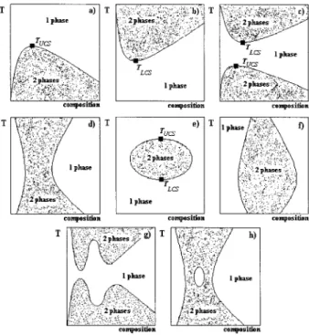
LLE in polymeric systems is usually repre-sented by an isobaric temperature versus compo-sition phase diagram, where compocompo-sition is nor-mally presented in terms of weight fraction, vol-ume fraction, or segment fraction. In Figure 1, we represent eight typical shapes of LLE phase dia-grams commonly found for polymeric systems, although they can be grouped in a lower number of distinct classes. Demixing in polymer solutions and blends may occur both upon cooling at low Correspondence to: L. P. N. Rebelo (E-mail: luis.rebelo@
dq.fct.unl.pt)
* Present address: Departamento de Engenharia Quı´mica, Universidade de Coimbra, Polo II, Pinhal de Marrocos, 3020 Coimbra, Portugal
Journal of Polymer Science: Part B: Polymer Physics, Vol. 38, 632– 651 (2000) © 2000 John Wiley & Sons, Inc.
temperatures (presenting an upper critical solu-tion temperature, UCST) [Fig. 1(a)], or upon heat-ing at high temperatures (presentheat-ing a lower crit-ical solution temperature, LCST) [Fig. 1(b)]. Most systems exhibit both UCST and LCST phase sep-aration [Fig. 1(c)]. In polymeric systems, this phase diagram is the rule rather than the excep-tion, and the individual appearance of only UCST or only LCST can be attributed either to experi-mental limitations or to difficulties in reaching metastable regions. In some special cases (non-theta, poor solvents), LCST and UCST can merge after reaching one point (called hypercritical tem-perature point) by searching for a convenient set of values of pressure, polymer molecular weight, and isotope substitution on the solvent or on the polymer [Fig. 1(d)]. These phase diagrams are usually referred as the “hourglass” type. Fre-quently, LCST lies above UCST, however. When specific interactions are present (e.g., hydrogen bonding in aqueous polymer solutions), a “closed-loop” phase diagram appears with the UCST lying above LCST [Fig. 1(e)]. Other types of unusual LLE phase diagrams can also be found in
poly-meric systems like those exhibiting a distorted “closed-loop” [Fig. 1(f)], bimodality [Fig. 1(g)], and miscibility “islands” [Fig. 1(h)]. Experimental ex-amples and theoretical predictions of the above-mentioned types have been compiled and stud-ied1,4,7–12in several works.
Certain variables such as pressure, polymer molecular weight, and isotope substitution, in ad-dition to other factors associated with polymer polymolecularity (polydispersity, tacticity, branch-ing, crosslinkbranch-ing, chain ending groups, etc.) may have a great effect (sometimes drastic) on poly-mer⫹ solvent and polymer ⫹ polymer miscibility. Because of this high complexity, phase equilib-rium behavior of polymeric systems and, particu-larly that of polymer ⫹ solvent systems, has drawn considerable attention from polymer phys-ical chemists and engineers and extensive work has been done concerning both theoretical and practical aspects during the last decades.
This work is part of a broad research program, which includes the experimental determination and the prediction and theoretical interpretation of liquid–liquid phase diagrams of polymer⫹ sol-vent systems, where the effects of MW, pressure, polydispersity, and isotope substitution are con-sidered. Very recently, we reported13 experimen-tal liquid–liquid cloud-point and spinodal data for polystyrene (PS)⫹ nitroethane systems as a func-tion of pressure, PS molecular weight and isotope substitution on PS and/or nitroethane.
In this article, we present a semiempirical phase equilibrium algorithm based on a modified Flory–Huggins model with a concentration- and temperature-dependent interaction parameter. It takes account of polymer polydispersity by using the methodology of Continuous Thermodynamics. This model, which is based on the work of Qian and collaborators,6,14 adds the methodology of Ratzsch and co-workers.15 The algorithm devel-oped herein permits us to portray commonly found polymer ⫹ solvent phase diagrams and to understand the effect of polydispersity on these diagrams. Using this algorithm and some robust fitting computer routines we have successfully modeled experimental data obtained for PS⫹ ni-troethane13 and, therefore, have obtained inter-action parameters directly from experimental LLE data.
The broader capabilities of the model have al-ready been demonstrated in a previous work,4 although the details of it were not presented there. This is done in the current work.
Figure 1. Types of LLE phase diagrams found for polymeric systems (polymer ⫹ solvent and polymer ⫹ polymer). (a) UCST type; (b) LCST type; (c) combined UCST⫹ LCST type; (d) “hourglass” type; (e) “closed-loop” type; (f) distorted “closed-“closed-loop” type; (g) bimodal combined UCST⫹ LCST type; (h) “hourglass” with a miscibility gap type. TUCSand TLCSare the upper and
MODELS FOR LLE IN POLYMER SOLUTIONS
The common problem to be solved when tackling LLE studies consists in determining at which set of conditions phase separation occurs. From a the-oretical point of view, this can be accomplished by searching the set of conditions where the second derivative of the Gibbs free energy of mixing in respect to composition is no longer positive (bor-derline between metastability and material insta-bility). For this purpose, it is necessary to achieve either an accurate expression for the excess Gibbs free energy or an equation of state (EoS). An optimum model or method should be capable of predicting and representing both VLE and LLE over a wide range of concentrations, pressures, and temperatures, and it should take polymer molecular weight and molecular weight distribu-tion into account. It should also have a reasonably small number of parameters, which should have physical meaning.
During the past decades, since the pioneering work of Chang,16 Flory,17 Huggins,18 and Gug-genheim19in the 1940s and 1950s, many thermo-dynamic theories and models of phase separation in polymeric systems (including solutions, blends, and melts) have been proposed and developed. Because of the different approaches and underly-ing theoretical backgrounds these theories and models have been classified in several distinct ways.
Following the classification proposed by Sara-iva,9,20two main different approaches can be con-sidered: (1) qualitative and/or semiquantitative descriptions of LLE in terms of polymer solubil-ity, where the main purpose is to predict whether or not a polymer is soluble in a certain solvent (or mixture of solvents) at certain conditions; (2) quantitative and qualitative descriptions of LLE, attempting to establish dependencies of LLE with temperature, composition, and pressure.
The first group of theories and models includes Hildebrand’s original solubility parameter theory and its extension to hydrogen bonding and polar compounds,21 the Shultz–Flory representation22 and other empirical predictive methods and “rules-of-thumb.”23
The second category is much more extensive. It comprises the classical Flory–Huggins model17,18 as well as its extensions and modifications;1,6,8,14,24 all the lattice-fluid (LF) based models and theo-ries (including the hole theory,25the mean-field-lattice-gas models,26 the well-known Sanchez–
Lacombe lattice-fluid EoS and derived models,27 and the cell theory28); all the perturbation theory based models (including the perturbed-hard-chain theory, PHCT, and the perturbed-soft-perturbed-hard-chain theory,29 PSCT, the statistical-associating-fluid theory,30SAFT, the perturbed-hard-sphere chain,31 PHSC, and the chain-of-rotators theory,32COR); the corresponding states EoS,33UNIFAC models,34 and UNIQUAC models.35 Recent models using a modified van der Waals EoS to polymer sys-tems9,36occur here as well.
Deveke,8Saraiva,9and Vimalchand and Dono-hue37have reviewed the main characteristics and applicability of some of these theories and models. These models have mostly been applied for the correlation and understanding of polymer solu-tions and blends. In many cases, the models are rather complex and their performance and predic-tive capabilities are not yet extensively investi-gated and exploited. So far, none of the available models are entirely engineering oriented, that is, both simple to apply and reasonably accurate and, therefore, have not been broadly used in polymer technology research and development. An important question remains: is there any good theory, or treatment, of solutions that can be both comprehensive in scope and accurate in its repre-sentation of equilibrium properties? Instead of seeking a theory, which is accurate in detail as well as comprehensive in scope, it may be more fruitful to adopt a simpler treatment of reason-able generality at the sacrifice of representation of individual cases.38 We decided to follow this last route and have adopted a semiempirical model based on the classical Flory–Huggins model but with a concentration- and tempera-ture- (and pressure-) dependent interaction pa-rameter.
The Classical Flory–Huggins Model: Background and Modifications
The well-known Flory–Huggins (FH) expres-sion17,18 for the Gibbs energy of mixing per vol-ume unit for a monodisperse polymer, B, in one single solvent, A, is given by:
⌬Gm RT ⫽ A VA lnA⫹ B VB lnB⫹AB (1)
where Viis the molar volume of component i,iis the volume fraction of component i, R is the gas constant, T is the absolute temperature, and
is the Flory–Huggins parameter, ⫽ FH/RT. In
the classical lattice FH model, FH is concentra-tion- and temperature-independent. This model contains many of the fundamentals of polymer solution phase equilibria but is not capable of describing, even qualitatively, the different types of phase diagrams found in polymer ⫹ solvent systems. One of these deficiencies is the inability to describe and explain the appearance of LCST curves. This fact is due to the incompressible na-ture of the model. Generally, with the exception of water, the free-volume percentage (or compress-ibility) of a low-molecular-weight compound is greater than the free-volume percentage of a mac-romolecule. In the case of polymer solutions, the difference in degree of thermal expansion be-tween polymer and solvent increases as temper-ature increases, attaining very high values as the temperature approaches the gas–liquid critical temperature of solvent. Phase separation is then induced by the expansion of the solvent that takes place with the consequent volume fluctuations. At these conditions, the extremely negative entropy of mixture (unfavourable effect) will overcome the negative value (favourable effect) of the enthalpy of mixture. Excess volumes of mixture are ex-pected to be negative39 providing dT/dp of the LCST transition is positive.40
As mentioned above, because of its simplicity this model displays several failures. It assumes that the FH interaction parameter is independent of concentration, temperature and pressure. How-ever, one knows from experiments that this is not true and it may depend, sometimes in a complex way, on these variables. To eliminate these limi-tations, several authors suggested the insertion, in a semiempirical way, of the concentration- and temperature-dependency in the FH interaction parameter. These empirically modified FH mod-els possess some theoretical background and their main advantage consists in their simplicity and ability to reproduce VLE and LLE experimental data (even for complex systems).41
Let us then write a more general expression for the Gibbs energy of mixing, per volume unit, for a monodisperse polymer, B, in one single solvent, A: ⌬Gm RT ⫽ A VA lnA⫹ B VB lnB⫹ g共B, T兲AB (2)
where the FH interaction parameter is now re-placed by a function of concentration and temper-ature, g(B, T). This dependence can be
consid-ered in many different ways.1,3–5,12,42 Following Orwoll,43the relation between the function, g(
B, T) and the FH interaction parameter,(B, T), is given by:
冕
B1
共, T兲 d ⫽ 共1 ⫺ B兲g共B, T兲 (3)
It is easy to show that these two functions,
g(B, T) and(B, T), only coincide when g(B, T)
is concentration-independent. Note that g(B, T)
is the mean value of(B, T) in respect to
concen-tration between ⫽ Band ⫽ 1. Combining eqs
2 and 3: ⌬Gm RT ⫽ A VA lnA⫹ B VB lnB⫹B
冕
B 1 共, T兲 d (4) The expressions for chemical potentials of compo-nents A and B can be easily derived:⌬A RT ⫽ln共1 ⫺B兲 ⫹B
冉
1⫺ VA VB冊
⫹共B, T兲VAB 2 (5) ⌬B RT ⫽lnB⫹ 共1 ⫺B兲冉
1⫺ VB VA冊
⫺ VBB共1 ⫺B兲共B, T兲 ⫹ VB冕
B 1 共, T兲 d (6) where ⌬ refers to the difference between the chemical potential in solution and that of the standard state. Now, according to the approach of Qian and co-workers,6,14 we can suppose that (B, T) is a function of a product between aconcentration function, B(B), and a temperature
function, D(T):
共B, T兲 ⫽ B共B兲D共T兲 (7)
One of the advantages of this approach is that one can find in the literature experimental inter-action parameter data (obtained by other meth-ods) and represent them as a function of temper-ature and concentration.43,44 The more realistic and applied forms for the functions B(B) and
D(T) are6,14,42 those where b
i and di are
adjust-able parameters: B共B兲 ⫽
冘
i⫽0 n biBi (8) D共T兲 ⫽ d0⫹ d1 T ⫹d2ln T (9) Under certain thermodynamic conditions, a ho-mogeneous polymer solution or mixture may sep-arate in two or more phases. The conditions for the equilibrium between two phases (marked as I and II) in a binary monodisperse component sys-tem (A and B) are expressed by the well-known identity of the chemical potentials of each species, A and B, between the distinct phases I and II:⌬AI ⫽ ⌬AII (10)
⌬BI ⫽ ⌬BII (11)
The manipulation of equations 5–11 reveals:
D共T兲A⫽ ln
冉
1⫺B II 1⫺BI冊
⫹ 共B II⫺ B I兲冉
1⫺VA VB冊
VA关B共BI兲BI 2 ⫺ B共BII兲BII 2 兴 (12) D共T兲B⫽ ln冉
B II BI冊
⫹ 共B I ⫺ B II兲冉
1⫺VB VA冊
VB冋
B共BII兲BII共1 ⫺BII兲 ⫺ B共BI兲BI共1 ⫺BI兲 ⫺冕
B II B I B共兲 d册
(13)We now proceed to consider the fact that D(T)A is equal to D(T)B, no matter the range of concen-trations considered.45 Thus, by simultaneously solving eqs 12 and 13 using a Newton–Raphson numerical method we obtain the coexistence curve. For a known volume fraction in phase I, B
I, we can calculate the volume fraction in phase
II, BII, which satisfies the relation of equality
between eqs 12 and 13. With this value, it is a straightforward matter to calculate the tempera-ture at which the two phases are in equilibrium.
The metastability limit of a binary mixture is defined by the spinodal curve, and can be thermo-dynamically defined by the stability criterion as46
⭸2共⌬G m/RT兲 ⭸A2 ⫽ ⭸2共⌬G m/RT兲 ⭸B2 ⫽ 0 (14)
The use of the stability criterion in eq 4 leads, then, to the spinodal curve equation:
1
VA共1 ⫺B兲 ⫹
1
VBB
⫺ D共T兲关2B共B兲 ⫹BB⬘共B兲兴 ⫽ 0 (15)
where the prime (⬘) denotes the first derivative of
B(B) in order toB.
The critical point of the binary mixture is the point at which cloud point and spinodal curves become identical. Thermodynamically it is de-fined by: ⭸2共⌬G m/RT兲 ⭸B2 ⫽ ⭸3共⌬G m/RT兲 ⭸B3 ⫽ 0 (16)
which is the same as saying: 1 共1 ⫺B兲 ⫹
冉
VA VB⫺ 1冊
⫺ D共T兲VAB关2B共B兲 ⫹BB⬘共B兲兴 ⫽ 0 (17) ⫺共1 ⫺1 B兲2⫹ D共T兲VA关2B共B兲 ⫹ 4B B⬘共B兲 ⫹B 2B⬙共 B兲兴 ⫽ 0 (18)where prime (⬘) and double prime (⬙) denote the first and the second derivatives, respectively, of
B(B) in respect to B. Solving simultaneously these two equations allow us to obtain the critical temperature(s), Tc, and the critical volume frac-tion,Bc.
This simple approach generates commonly found LLE phase diagrams of monodisperse poly-mer⫹ solvent and polymer ⫹ polymer systems as well as other unusual types of phase diagrams like those with occurrence of multiple critical points, coalescence of cloud-point curves, and the appearance of bimodality in cloud-point and spi-nodal curves.4,6,14,47This can be done by choosing the appropriate magnitudes and signs of the pa-rameters, biand di. However, when modeling
ex-perimental data, some care has to be taken, espe-cially when extrapolating beyond the experimen-tal fitted range.
A Continuous Polydisperse Thermodynamic Modified Flory–Huggins Model
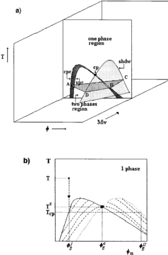
All the material above described considers the polymer to be monodisperse, therefore truly bi-nary mixtures. However, polymers do not have a well-defined molecular weight but a range (distri-bution) of molecular weights (polydispersity). Therefore, a solution of one polymer in one single solvent does not behave as a true binary mixture but as a multicomponent system of species chem-ically similar but differing in the polymerization degree. Usually these systems are described as quasibinary or pseudobinary. Polymer polydis-persity might have a large effect in the thermo-dynamic properties and in LLE of polymer solu-tions.1,15,47,48For example, the binodal curve of a true binary polymer ⫹ solvent system splits in three different kinds of curves if the system is considered as polydisperse: a cloud-point curve, a “shadow” curve and an infinite number of coexist-ence curves.15 This is illustrated in Figure 2. Starting from the homogeneous region, at a given temperature, T, and composition, BI, upon
de-creasing temperature until reaching the cloud-point curve, at Tcp, the (overall) polymer content of the first droplets of the precipitated phase does not correspond to a point on the cloud-point curve but to a corresponding point on the shadow curve, B
II. Upon lowering temperature further, the
equi-librium phases change their compositions neither according to the cloud-point curve nor to the shadow curve but rather according to the related branches of the coexistence curves. These are di-vided in two branches and just one of them is continuous: the one passing through the critical point. At this point, the cloud-point curve, the shadow curve and the spinodal curve (not repre-sented on Fig. 2) intersect. Thus, the critical point does not correspond to the maximum of the cloud-point curve (as is the case for strictly binary sys-tems).
This complicated behavior is due to polymer polydispersity. Polymers in coexisting phases also present different mean molecular weights distri-butions and, therefore, may present distinct mo-lecular weight distributions. The cloud-point curve always refers to both the molecular weight and molecular weight distribution of the initial polymer but this does not occur with the first
droplets formed on the shadow curve. Such drop-lets contain polymer with different molecular weight (and molecular weight distribution) from the initial polymer.
Let us consider now that polymer, B, is poly-disperse. Equation 4 should be rewritten:
⌬Gm RT ⫽ A VA lnA⫹
冘
i⫽1 n Bi VBi lnBi ⫹B冕
B 1 共, T兲 d (19) Figure 2. (a) Typical LLE phase diagram in the (T,,MW) space at constant pressure for a polydisperse
poly-mer⫹ solvent. Spc is the spinodal curve. Cpc is the cloud-point curve. Cp is the critical point. Shdw is the shadow curve. A is in equilibrium with C and and B is in equilibrium with D. (b) T,Bprojection of a
polydis-perse system at constant pressure. (—) Cloud-point curve; (䡠 䡠 䡠) shadow curve; (- - -) coexistence curves; (■) critical point.
where Vbi and Bi are, respectively, the molar volume and the volume fraction of component i of polymer B.Bis the total volume fraction of poly-mer B. Polydispersity effect does not have a sig-nificant effect on the interaction parameter,49 (B, T), and thus its effect it is not considered in
the last term of eq 19. The equilibrium conditions between two phases, denoted as I and II, are given by:
⌬AI ⫽ ⌬AII (20)
⌬BiI ⫽ ⌬BiII, 1ⱕ i ⱕ n 共n equations兲 (21)
and the resolution of the equilibrium criteria be-comes impracticable because of the very high number of equations involved, (n⫹ 1).
Therefore, in this work we decided to introduce the methodology of Continuous Thermodynamics into the model described above.10,47This method is highly useful in the thermodynamic treatment of polydisperse systems like crude oils and deriv-atives, vegetable oils and synthetic polymers. In the referred cases, “polydisperse” means that these systems possess a great number of chemi-cally similar species differing just in the molecu-lar weight of the components. Some particumolecu-lar applications have been developed during the last decades but only recently have the fundamentals of Continuous Thermodynamics been well-estab-lished50and the advantages of the method recog-nized.1,51
Following Ratzsch and co-workers,15which de-veloped the application to LLE of polymer⫹ sol-vent systems, let us rewrite10,47eq 19:
⌬Gm RT ⫽ A rA lnA⫹
冕
BWB共r兲 r ln共BWB共r兲兲 dr ⫹B冕
B 1 共, T兲 d (22) where⌬Gmis now the Gibbs energy of mixing but per segment unit, A and B are the segment fractions of solvent A and polymer B, respectivelyrAis the solvent segment number (usually consid-ered as unity, since it is assumed that a solvent molecule has the same size of a polymer mono-meric unit) r is the segment number and WB(r) is the continuous and intensive distribution func-tion of polymer segment number. Once again, the polydispersity effect is not considered in the
in-teraction parameter, (B, T), and is thus not a function of the segment number r.
The expressions for chemical potentials of com-ponents A and B can again be derived, resulting in: ⌬A RT ⫽ln共1 ⫺B兲 ⫹
冉
1⫺ rA r冊
⫹ rAB2共B, T兲 (23) ⌬B共r兲 RT ⫽ ln关BWB共r兲兴 ⫹冉
1⫺ r r冊
⫺ rB共1 ⫺B兲共B, T兲 ⫹ r冕
B 1 共, T兲 d (24) where r is the number-average segment number for the considered phase (I or II), defined as:151 r ⫽ A rA⫹ B rB (25) 1 rB⫽
冕
WB共r兲 r dr (26)Here, rBis the number-average segment
num-ber of polymer, B, and for the considered phase. The equilibrium conditions between two phases, denoted as I and II, will be given by:
⌬A I ⫽ ⌬ A II (27) ⌬B I共r兲 ⫽ ⌬ B II共r兲 (28)
These conditions lead to the new equations:
D共T兲 ⫽ ln
冉
1⫺B II 1⫺BI冊
⫹B II冉
1⫺rA rBII冊
⫺B I冉
1⫺rA rBI冊
rA关B共BI兲BI 2 ⫺ B共BII兲BII 2 兴 (29) D共T兲 ⫽ ln冉
B IIW B II共r兲 BIWBI共r兲冊
⫹ r冋
BII⫺BI rA ⫹ BI r BI ⫺ BII rBII册
r冋
B共BII兲BII共1 ⫺IIB兲 ⫺ B共BI兲BI共1 ⫺BI兲 ⫺冕
B II B I B共兲 d册
(30)If one assumes the distribution function, WB(r), to be of the Schulz–Flory type, for each phase, one has: WB共r兲 ⫽ kk⫹1 rB⌫共k ⫹ 1兲
冉
r rB冊
k exp冉
⫺k r rB冊
(31)where ⌫ is the Gamma Function (defined in its usual mathematical terms). k is defined by:
k⫽ 1
⫺ 1 (32)
where is the polymer polydispersity index, which, in turn, is defined by:
1 ⫽ rB rBw⫽ 2 ⫺ rBz rBw (33)
where rBw and rBz, are, respectively, the
weight-average segment number and the z-weight-average seg-ment number for polymer B and for the consid-ered phase. On the other hand:
rB⫽ Mn Ms ; rBw⫽ Mw Ms (34)
where Mnis the polymer number-average
molec-ular weight, Mw is the polymer weight-average
molecular weight, and Msis the molecular weight
of one monomer unit.
For this distribution function, and under cer-tain restritions,15it is possible to obtain the sym-metry relation: BII 共rBII兲k⫹1⫽ BI 共rBI兲k⫹1 (35)
Application of eqs 31–35, permits us to solve eq 29 and 30, and therefore obtain the cloud-point and shadow curves.
Other types of polymer distribution functions (different from the Schultz–Flory distribution function) are possible but it could not be possible to do certain simple analytical and mathematical procedures conducing to a symmetry relation like the one expressed by eq 35. This relation greatly simplifies the phase equilibrium algorithm.
In a manner similar to the above-described monodisperse case, one can obtain the spinodal curve equation: 1 rA共1 ⫺B兲 ⫹ 1 r BwB ⫺ D共T兲关2B共B兲 ⫹BB⬘共B兲兴 ⫽ 0 (36) Eq 36, together with eq 37, ⫺r 1 A共1 ⫺B兲2⫹ rBz r Bw2 B2 ⫹ D共T兲关3B⬘共B兲 ⫹BB⬙共B兲兴 ⫽ 0 (37)
define the critical point of the mixture.
DISCUSSION
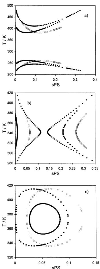
With these two models at hand, one considering the polymer as monodisperse and the other as polydisperse, it is possible to study the effect of polydispersity on LLE phase diagrams. Figure 3(a) illustrates this effect for a UCST type of phase diagram. Polymer polydispersity decreases the miscibility of the system, increasing the tem-perature of the cloud-point curve. Shadow and spinodal curves are also represented. As men-tioned above, the critical point does not corre-spond to the cloud-point maximum (in the poly-disperse case). In Figure 3(b), only cloud-point curves are represented for several distinct values of polydispersity index, . As expected, an in-crease in polydispersity corresponds to a miscibil-ity decrease. It is not presented here, but this polydispersity effect is larger for greater polymer molecular weights. The number-average molecu-lar weight and all parameters used are the same in all cases, monodisperse and polydisperse. The monodisperse model presented above was slightly modified in order to also use polymer segment fractions. In Figure 4, the polydispersity effect on commonly found phase diagrams for polymer ⫹ solvent systems is represented. In some cases, polydispersity has a drastic effect on LLE and miscibility decrease is a commonly found charac-teristic in all cases presented.
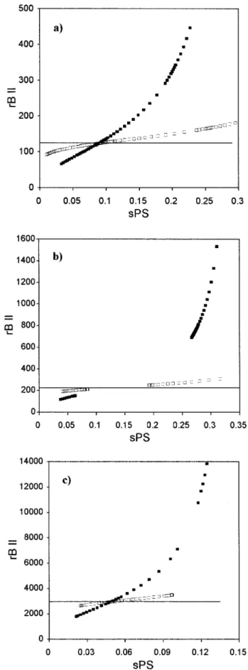
In Figure 5 we represent the number-average segment number of the precipitated phase (phase II), rBII, as a function of the polymer segment
frac-tion of the shadow curve, sPS, for different poly-dispersity indexes, and for the examples pre-sented in Figure 4. The polymer precipitated in phase II does not have the same number-average molecular weight (and consequently the same number-average segment number) of the polymer
in the initial phase (phase I), except at the critical point. These differences between the number-av-erage segment numbers of phases I and II in-crease with increasing polydispersity. The possi-bility of polymer fractionation by equilibrium and
phase separation has been known for a long time. One concludes that this model permits us to un-derstand and quantify polymer fractionation due to phase precipitation.
The Polystyreneⴙ Nitroethane Example
Detailed experimental cloud-point and spinodal data for polystyrene⫹ nitroethane systems have been reported in a previous work.13With the mod-els described above (monodisperse and polydis-perse), we can obtain the concentration- and tem-perature-dependent interaction parameters of the referred systems. In addition, their shifts due to variation of pressure, MW, and isotope content can be revealed by an appropriate least-squares fit to experimental cloud-point data, adjusting the
biand diparameters. The functional form of the
interaction parameter is given by:
共B, T兲 ⫽ B共B兲D共T兲 ⫽ 共b0⫹ b1B⫹ b2B
2
⫹ b3B3⫹ b4B4兲
冉
d0⫹d1
T ⫹d2ln共T兲
冊
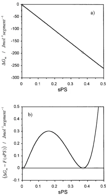
(38) In Tables I and II, we report these fitted pa-rameters for eight polystyrene⫹ nitroethane sys-tems experimentally studied, at two nominally different pressures, 0.0 and 4.0 MPa, and for the monodisperse and polydisperse cases, respec-tively. With these adjusted parameters we have calculated spinodal curves, critical temperatures, and critical segment fractions. The latter two quantities are also reported in Tables I and II. For all these systems we have considered: b0 ⫽ 1; b3 ⫽ 0; b4⫽ 0; d2 ⫽ 0Number-average molecular weight values and polydispersity indexes were supplied by polysty-rene manufacturers and have been reported else-where.13Nominal values of MW for each studied system as well as polydispersity indexes are found in the tables13. Experimental PS weight fractions were converted to PS segment fractions. In Figure 6(a), the Gibbs free energy of mixing per segment unit,⌬Gm, is plotted as a function of polystyrene segment fraction, sPS. We also repre-sent the coexistence equilibrium segment frac-tions obtained from identical chemical potentials of each component in the two coexisting phases. The figure clearly shows that it is impossible to graphically detect these points in a ⌬Gm curve. The apparent linearity observed in Figure 6(a) is a special and typical feature of LLE of polymer solutions. To identify the hidden curvatures of Figure 3. Polydispersity effects on UCST
liquid–liq-uid phase diagrams. (a) Typical polydispersity effect. (F) Cloud-point curve (monodisperse); (E) spinodal curve (monodisperse); (■) cloud-point curve (polydis-perse, ⫽ 1.50); (䊐) shadow curve (polydisperse, ⫽ 1.50); (‚) spinodal curve (polydisperse, ⫽ 1.50); (¨) critical point (monodisperse and polydisperse). (b) Poly-dispersity effect on cloud-point curves. (■) Cloud-point curve (monodisperse); (䊐) cloud-point curve (polydis-perse, ⫽ 1.05); (F) cloud-point curve (polydisperse, ⫽ 1.10); (E) cloud-point curve (polydisperse, ⫽ 1.50); (¨) critical point (monodisperse and polydisperse). Used parameters: b0⫽ 1.0, b1⫽ 0.2, b2⫽ 0.0; d0⫽ ⫺0.6, d1
⌬Gm curves, in Figure 6(b) one represents the
difference between⌬Gmand the straight line re-sulting from the connection between the points of stable coexistence equilibrium,9⌬G
m⫺ F(sPS), as
a function of sPS. This new function permits the clear graphical identification of both the inflection points (spinodal) and minima (binodal).
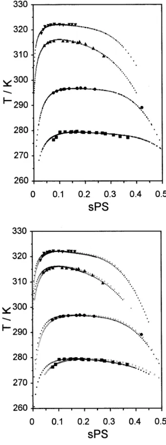
In Figure 7, modeled LLE phase diagrams are presented together with experimental data for systems I–IV, at 4.0 MPa, considering mono and polydisperse cases. This figure corresponds to the polystyrene molecular weight effect analysis of LLE. Both models conform very well to the exper-imental cloud-point data. Because of the low poly-dispersity of our polystyrene samples (we have used polystyrene standards of well-defined molec-ular weights), modeled cloud-point and shadow curves do not differ much. Fitted biand di param-eters are also not very different in the two ap-proaches (mono and polydisperse). This can be seen in Figure 8 where we can observe the effect of polymer molecular weight on the fitted param-eters. Generally speaking, with increasing molec-ular weight (and the consequent decrease in mis-cibility, and critical concentration), the b1 param-eter increases, b2decreases, d0increases initially and then stays approximately constant and d1 decreases initially and then also keeps roughly constant.
Comments on the Pressure Dependence of Parameters and Their Physical Meaning
It has very recently been shown40that the sim-plest excess Gibbs energy model capable of repre-senting all types of basic LL phase diagrams and all their possible general pressure dependencies is one corresponding to eq 38 in which d0 is a linear function of pressure, d1 has a quadratic
Figure 4. Polydispersity effects on other liquid– liquid phase diagrams. Comparison between monodis-perse and polydismonodis-perse systems. (F) Cloud-point curve (monodisperse); (■) cloud-point curve (polydisperse, ⫽ 1.50); (䊐) shadow curve (polydisperse, ⫽ 1.50). (a) Combined UCST ⫹ LCST type. Used parameters: b0
⫽ 1.0, b1⫽ 0.2, b2⫽ 0.0; d0⫽ ⫺6.8829, d1⫽ 345.5, d2
⫽ 1.1; Mn⫽ 13,000; Ms⫽ 104; rA⫽ 1. (b) “Hourglass”
type. Used parameters: b0⫽ 1.0, b1⫽ 0.653, b2⫽ 0.0; d0
⫽ ⫺6.9933, d1⫽ 376.2, d2⫽ 1.1; Mn⫽ 23500; Ms⫽ 104;
rA ⫽ 1. (c) “Closed-Loop” type. Used parameters: b0
⫽ 1.0, b1⫽ 0.65, b2⫽ 0.0; d0⫽ 2.582; d1⫽ ⫺ 111.9, d2
dependence on it, and d2 is a constant. In other words, 共B, T, p兲 ⫽ B共B兲D共T, p兲 ⫽ B共B兲 ⫻
冉
c⫹ b1p⫹ 共a0⫹ a1p⫹ a2p2兲 T ⫺ c0ln共T兲冊
/R (39) An expression such as that given by eq 39 can generate all four basic types of (T,p) critical loci including some that have never been experimen-tally proven.40 It is a straightforward matter to show that the underlying excess properties such as the excess volume and excess enthalpy are given, respectively, by:E共
B, T, p兲 ⫽ B共B兲共a1⫹ 2a2p⫹ b1T兲 (40)
hE共
B, T, p兲 ⫽ B共B兲共a0⫹ a1p⫹ a2p2⫹ c0T兲 (41)
The excess volume of the solution should thus be linear in pressure and temperature, whereas the excess enthalpy has to have a quadratic depen-dence on pressure. The ratio between these two excess functions multiplied by the temperature of critical demixing reveals the numerical value for the pressure dependence of the locus of critical temperature. On the other hand, some parame-ters in equations (38 – 41) have a direct physical meaning. While d2 and c0 define the excess heat capacity, Cp
E
⫽ c0B(⌿B)⫽ ⫺R d2B(⌿B), b1and a2
Figure 5. Polydispersity effect on the shadow curve number-average segment number (rB II) as a function of the segment fraction of polymer (sPS) in the shadow curve. Comparison between monodisperse and polydis-perse systems. (Solid line) Number-average segment number, polymer B, phase I, cloud-point curve, mono-disperse; (■) number-average segment number, poly-mer B, phase II, shadow curve, ⫽ 1.50; (䊐) number-average segment number, polymer B, phase II, shadow curve, ⫽ 1.10. (a) Combined UCST ⫹ LCST type. Used parameters: b0 ⫽ 1.0, b1⫽ 0.2, b2⫽ 0.0; d0
⫽ ⫺6.8829, d1⫽ 345.5, d2⫽ 1.1; Mn⫽ 13,000; Ms⫽104;
rA⫽ 1. (b) “Hourglass” type. Used parameters: b0⫽ 1.0, b1 ⫽ 0.653, b2 ⫽ 0.0; d0 ⫽ ⫺6.9933, d1 ⫽ 376.2, d2
⫽ 1.1; Mn⫽ 23,500; Ms⫽ 104; rA⫽ 1. (c) “Closed-loop”
type. Used parameters: b0⫽ 1.0, b1⫽ 0.65, b2⫽ 0.0; d0
⫽ 2.582, d1⫽ ⫺111.9, d2⫽ ⫺0.3; Mn ⫽ 140,000; Ms
are closely related to the excess thermal expan-sivity and compressibility. Parameters a1 and a0 refer, respectively, to the values of the excess volume and excess enthalpy in a hypothetical state at null temperature and pressure.
Because of the small pressure effect on the phase diagrams of (nitroethane ⫹ polystyrene), which amounts to about 0.1– 0.3 K/MPa at our experimental conditions, it was not possible to accurately define the pressure dependence of pa-rameters d0and d1(see also Tables I and II) in eq 38. Optimally, one should work near temperature hypercritical points (where dTc/dp tends to infin-ity) or substantially augment the range of studied pressures.
Isotope Effects on the Polystyrene
ⴙ Nitroethane System
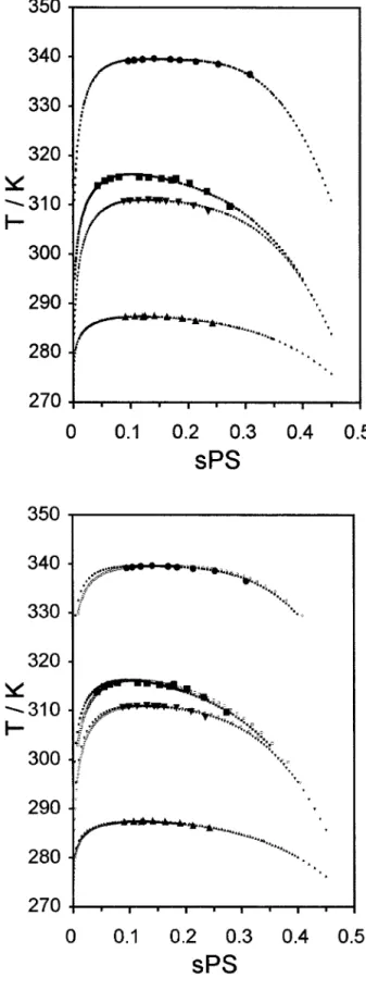
In Figure 9, we represent experimental and mod-eled LLE phase diagrams for some polystyrene ⫹ nitroethane systems, at 4.0 MPa, (Systems III, V, VI, and VII) corresponding to systems
contain-ing samples with similar polystyrene number-av-erage molecular weight (Mn ⬃ 90,000) but with isotope substitution in polystyrene and/or nitro-ethane. Monodisperse and polydisperse case fits are presented. Isotope substitution on polysty-rene (system VI) increases miscibility, whereas isotope substitution on nitroethane (system V) decreases it. Simultaneous deuteration on poly-styrene and nitroethane (system VII) does not change remarkably phase equilibrium when com-pared with the case where both species are pro-tonated (system III). For all these systems, the parameters, b1 and b2, do not change markedly with isotope substitution nor do parameters d0 and d1 vary a lot, except for system VI. These observations are valid for both the monodisperse and polydisperse approaches (see Tables I and II). Van Hook and collaborators1,2,52 have pub-lished cloud-point and spinodal data on systems containing polystyrene (perprotonated and per-deuterated) in several solvents (acetone, methyl-cyclopentane, and propionitrile), also protonated and deuterated. They developed a first-order in-Table I. Modeling Results for Atactic Polystyrene⫹ Nitroethane Systems: Monodisperse Casea
4.0 MPa Systemb b 0 b1 b2 d0 d1 Bc Tc(K) I 1.0000 0.11585 1.25423 0.35535 59.35046 0.165 279.379 II 1.0000 0.33425 1.09351 0.44152 27.26491 0.159 296.699 III 1.0000 0.49725 0.85068 0.42142 29.41000 0.102 316.207 IV 1.0000 0.51290 0.89042 0.43094 25.86470 0.099 322.099 V 1.0000 0.48376 0.94567 0.45335 20.71253 0.143 339.501 VI 1.0000 0.52850 0.77768 0.22780 82.10817 0.120 287.454 VII 1.0000 0.49071 0.89716 0.43463 24.99186 0.125 311.014 VIII 1.0000 0.30899 1.06937 0.13776 107.99653 0.146 269.219 0.0 MPa Systemb b 0 b1 b2 d0 d1 Bc Tc(K) I 1.0000 0.12416 1.24015 0.44427 35.09139 0.166 279.808 II 1.0000 0.33324 1.09543 0.44381 26.66198 0.159 297.322 III 1.0000 0.50336 0.83392 0.42423 28.53345 0.103 317.315 IV 1.0000 0.51571 0.87922 0.43216 25.55090 0.098 323.458 V 1.0000 0.48640 0.93901 0.45041 21.76868 0.142 341.108 VI 1.0000 0.53026 0.77546 0.22518 83.03379 0.121 288.167 VII 1.0000 0.49065 0.89798 0.43306 25.55727 0.126 311.988 VIII 1.0000 0.30898 1.06941 0.13855 107.92576 0.146 269.570
aParameters of eq 38. The subscript c refers to critical conditions. bSystem I: a-PS(h
8)-13000⫹ h5-nitroethane; System II: a-PS(h8)-30000⫹ h5-nitroethane; System III: a-PS(h8)-90000⫹ h5
-nitroethane; System IV: a-PS(h8)-130000⫹ h5-nitroethane; System V: a-PS(h8)-90000⫹ d5-nitroethane; System VI: a-PS(d8)-90000
terpretation of phase equilibrium isotope substi-tution effect, which combines the main features of the Guggenheim’s symmetrical mixtures theory53 and the statistical theory of condensed phase iso-tope effects.54Here, we adopt the simplest form of the classical FH model, that is, considering a monodisperse polymer, B, and that the interac-tion parameter, FH, is concentration- and tem-perature-independent. This results for the excess Gibbs energy in:
⌬Gexc⫽
FHB共1 ⫺B兲 (42)
At critical concentration, demixing occurs when-ever
FH
RT ⱖ2 (43)
Therefore,
RTc⫽FH/2 (44)
The expressions for chemical potentials of com-ponents A and B will be:
⌬A RT ⫽ln共1 ⫺B兲 ⫹B
冉
1⫺ rA rB冊
⫹ 2rAB 2 (45) ⌬B RT ⫽ln共B兲 ⫹ 共1 ⫺B兲 ⫻冉
1⫺rB rA冊
⫹ 2rB共1 ⫺B兲 2 共46兲The major contribution for the isotope effect1,54 comes from the zero-point energy term (B term of Bigeleisen’s AB equation54): ␦⌬0⬁ RT ⫽ A T2⫹ B T (47) A⫽ 1 24
冉
hc k冊
2冘
i 关共⬘i2⫺i2兲⬁⫺ 共⬘i2⫺i2兲0兴 (48)Table II. Modeling Results for Atactic Polystyrene⫹ Nitroethane Systems: Polydisperse Casea
4.0 MPa Systemb b 0 b1 b2 d0 d1 Bc Tc(K) I 1.0000 0.19170 1.13386 0.27015 81.27313 0.180 279.521 II 1.0000 0.35613 1.05616 0.41632 34.22106 0.170 296.774 III 1.0000 0.50706 0.81829 0.40189 35.40242 0.102 316.254 IV 1.0000 0.51083 0.89948 0.43667 24.01365 0.099 322.147 V 1.0000 0.50378 0.90102 0.38578 43.24158 0.148 339.585 VI 1.0000 0.53534 0.75756 0.19993 90.00599 0.119 287.460 VII 1.0000 0.49883 0.87587 0.41964 29.49931 0.126 310.999 VIII 1.0000 0.30315 1.08290 0.17679 97.49265 0.145 269.209 0.0 MPa Systemb b 0 b1 b2 d0 d1 Bc Tc(K) I 1.0000 0.19084 1.13550 0.27256 80.71305 0.180 279.857 II 1.0000 0.35422 1.05972 0.42012 33.20122 0.169 297.400 III 1.0000 0.51399 0.79932 0.39372 38.01322 0.103 317.292 IV 1.0000 0.51328 0.88952 0.43801 23.65634 0.098 323.511 V 1.0000 0.50647 0.89341 0.38881 42.35891 0.145 341.090 VI 1.0000 0.53737 0.75480 0.19679 91.09714 0.120 288.173 VII 1.0000 0.49897 0.87631 0.41755 30.23909 0.126 311.978 VIII 1.0000 0.30309 1.08304 0.17782 97.34170 0.145 269.554
aParameters of eq 38. The subscript c refers to critical conditions. bSystem I: a-PS(h
8)-13000⫹ h5-nitroethane; System II: a-PS(h8)-30000⫹ h5-nitroethane; System III: a-PS(h8)-90000⫹ h5
-nitroethane; System IV: a-PS(h8)-130000⫹ h5-nitroethane; System V: a-PS(h8)-90000⫹ d5-nitroethane; System VI: a-PS(d8)-90000
B⫽1 2
冉
hc k冊
冘
j 关共⬘j⫺j兲⬁⫺ 共⬘j⫺j兲0兴 (49)where k is the Boltzmann’s constant; h, the Planck’s constant; c, the velocity of light; and , the wave number. In this case, “⬘” denotes the lighter isotope. The above equations can be ap-plied when the isotope-sensitive vibrations of the
considered molecules fall in two classes: (1) a high-frequency set (indexed over j), which can be treated by the zero-point energy (ZPE) approxi-mation (B term); and (2) a low-frequency set (in-dexed over i), which includes the external vibra-tions (hindered translation and rotation), and the internal rotations. This last set can be treated by the high-temperature approximation (A term).
Let us then consider that the major portion of the isotope effect is due to the B term (ZPE), associated with the carbon– hydrogen (COH) or the carbon– deuterium (COD) stretching modes, when the molecule is transferred from its pure reference state, o, to infinite dilution in the other component of the mixture, ⬁. This way, we can calculate the free transfer energy between these two states.
The transfer from a perprotonated reference state to a perdeuterated solvent state, leads to a transfer energy of:
␦⌬Ac⫽ 共⌬Ac兲perdeuterated⫺ 共⌬Ac兲perprotonated (50) On the other hand, the transfer from a perpro-tonated reference state to a perdeuterated poly-mer (solute) state, leads to a transfer energy:
␦⌬Bc⫽ 共⌬Bc兲perdeuterated⫺ 共⌬Bc兲perprotonated (51) Considering: ␦⌬Ac⫽ 1 2nAcrA␦⌬0⬁Nhc (52) ␦⌬Bc⫽ 1 2nBcrB␦⌬0 ⬁Nhc (53)
it is possible to obtain the vibrational frequency shifts,␦⌬0⬁, associated with the considered isoto-pic substitution. In this case, nicis the number of COH oscillators in a solvent molecule (A) or in a polymer segment (B). riis the segment number of solvent (A) or polymer (B) and, N is the Avo-gadro’s number.
Usually, the typical isotope effect for the COH stretching vibration, in the pure liquid state, is of the order of 800 cm⫺1and the typical frequency shift for the COH and COD stretchings for the liquid– gas phase transition is of the order of 10 –14 cm⫺1. This latter value is comparable to the value of transferring one molecule from its pure reference state to infinite dilution in another component.54
Figure 6. (a) ⌬Gm versus sPS curve obtained with
the fitted parameters for system III, at 0.0 MPa and 299.26 K (monodisperse model). (—)⌬Gm versus sPS
curve; (E) points of stable phase equilibrium. (b)⌬Gm
F(sPS) versus sPS curve obtained with the fitted
pa-rameters for system III, at 0.0 MPa and 299.26 K (monodisperse model). (—) ⌬Gm F(sPS) versus sPS
Using the above equations and applying them to the systems studied experimentally, reveals that the isotope effect observed for systems III and V [a-PS(h8)-90000/h5-nitroethane and a-PS(h8)-90000/d5-nitroethane] corresponds to a blue shift of the order of 1.2–1.3 cm⫺1for each one of the five COH stretches in the nitroethane mol-ecule. For the polystyrene⫹ acetone system,1 iso-topic substitution on acetone corresponds to a blue shift of the order of 9 cm⫺1for each one of the six COH stretches in the acetone molecule. In the case of other systems1 such as polystyrene ⫹ methylcyclopentane and polystyrene ⫹ propi-onitrile this blue shift is of the order of 2 cm⫺1and 39 cm⫺1, respectively, for each one of the COH stretches in the solvent molecule.
In the same way, for the systems III and VI [a-PS(h8)-90000/h5-nitroethane and a-PS(d8 )-90000/h5-nitroethane], the observed isotope effect corresponds to a red shift of the order of 3.2–3.3 cm⫺1for each one of the eight COH stretches in a polystyrene segment (considered as a monomer molecule, i.e., styrene.). In the case of the polysty-rene ⫹ acetone system, isotopic substitution of polystyrene corresponds to a red shift of the order of 7 cm⫺1for each one of the eight COH stretches in a polystyrene segment. For polystyrene ⫹ methylcyclopentane and polystyrene ⫹ propion-itrile, this red shift is of the order of 0.5 cm⫺1and 4 cm⫺1, respectively, for each one of the eight COH stretches in a polystyrene segment. For sys-tems II and VIII [a-PS(h8)-30000/h5-nitroethane and a-PS(d8)-26600/h5-nitroethane], isotopic sub-stitution on polystyrene corresponds to a red shift of the order of 2.8 –2.9 cm⫺1 for each one of the eight COH stretches in a polystyrene segment.
It should be noted that larger shifts are ex-pected to be found in systems experiencing ther-modynamic conditions close to hypercritical points, such as those occurring in acetone or
pro-Figure 7. Experimental and modeled LLE phase di-agrams for some polystyrene ⫹ nitroethane systems (Systems I-IV). Molecular weight effect at 4.0 MPa. Monodisperse (upper) and polydisperse (lower) cases.
(■) Experimental cloud-point, Syst. I: a-PS(h8
)-13000; (F) experimental cloud-point, Syst. II: a-PS(h8
)-30000; (Œ) experimental cloud-point, Syst. III: a-PS(h8
)-90000; () experimental cloud-point, Syst. IV: a-PS(h8
)-130000; (■) cloud-point, modeled, Syst. I: a-PS(h8)-13000;
(F) cloud-point, modeled, Syst. II: a-PS(h8)-30000; (Œ)
cloud-point, modeled, Syst. III: a-PS(h8)-90000; ()
cloud-point, modeled, Syst. IV: a-PS(h8)-130000; (䊐) shadow,
modeled, Syst. I: a-PS(h8)-13000; (E) shadow, modeled,
Syst. II: a-PS(h8)-30000; (‚) shadow, modeled, Syst. III:
a-PS(h8)-90000; (ƒ) shadow, modeled, Syst. IV: a-PS(h8
pionitrile. Here, the mixture should experience a large (negative) excess volume.40 In contrast, phase equilibria of solutions of polystyrene in methylcyclopentane or nitroethane show subtle pressure dependence and, consequently, isotope effects are small.
Some Remarks
The main goal of this article is to present in detail an accurate and efficient methodology capable of dealing with all kinds of behavior presented by liquid–liquid equilibrium in polymeric systems, be they of the monodisperse or polydisperse type. Ways of extending the treatment in order to in-clude pressure and isotope effects are also ex-plained. Since we have clearly demonstrated that the model is completely, generally applicable [see, e.g., Figs. 4 and 5, (a– c)], we decided to focus on the main goal and present just one set of real (closely related) systems. The reason for choosing PS ⫹ nitroethane as an example of practical ap-plicability is twofold. First of all, very recently these systems were studied in this laboratory13 and their raw data published without any theo-retical modeling. Furthermore, the set of systems comprised by applying pressure and isotope ef-fects to PS ⫹ nitroethane constitutes a nonspe-cific and possible model case for the most common experimentally found behavior (UCST type). This is well illustrated in Figures 7 and 9, and Tables I and II. Pressure and isotope effects, as well as polymer molecular weight, induce a change in solvent’s quality similar to that obtained by its real substitution. In other words, plots like those represented in Figures 7 and 9 could represent the same kind of systems, or not.
Although the detailed description of this meth-odology has never been previously presented, its application to other specific systems has been suc-cessfully checked in preliminary tests. Examples include the very unusual behavior (strongly bi-modal) of PS⫹ acetaldehyde,4PS⫹ methylcyclo-pentane10 or PS ⫹ acetone.47 As new relevant systems become experimentally available, we in-tend to apply the algorithm herein described in an improved version where pressure is directly taken into account as suggested by eqs 39 – 41. Luszczyk et al.1 have reviewed the pertinent literature of modeling pseudobinary mixtures. All those meth-ods referred therein differ in the type of chain-distribution assumed for the polymer, in regard to the model for calculation of multicomponent ac-tivity coefficients (and their temperature and pressure dependence), and the numerical strat-egy applied. The qualities that distinguish this algorithm from others have to do with its very fast numerical convergence, very high precision, and use of a functional temperature6,14and pressure (this work, eqs 39 – 41) form for activity coeffi-cients with obvious meaningful physical mean-Figure 8. Fitted bi(case a) and di(case b) parameters
for some polystyrene⫹ nitroethane systems (systems I–IV). Molecular weight effect at 4.0 MPa. Monodis-perse and polydisMonodis-perse cases. ( ) b2, d1,
monodis-perse; ( ) b1, d0, monodisperse; ( ) b2, d1,
ing.40 The use of a standard Newton–Raphson numerical methodology for solving simulta-neously eqs 12 and 13, or 21 and 30 in conjunction with eq 9 through a Borland Pascal program per-mits us to work at double-precision. Typically, the ultimate increment net is of the order of 10⫺9in the D(T) functions when searching for solutions in , and of the same magnitude for T (through eq 9). It is thus possible to use directly the algorithm within a large range of molecular weights and polydispersity indexes without any additional effort.
Finally, we turn now our attention to a brief discussion about comparisons between the mono-disperse and polymono-disperse cases. So far, and throughout the text, comparisons between cases of ⫽ Mw/Mn⫽ 1 and ⬎ 1 have been made at
fixed Mn. In other words, when comparing the two cases, the value for Mw in the polydisperse solu-tion is greater than that of the monodisperse. As can be seen from analysis of Figures 3 and 4, the effective effect of polydispersity corresponds to one where miscibility decreases. In a UCST type of behavior this translates as follows: as the de-gree of polydispersity increases, the spinodal moves towards higher temperatures, the critical point to higher temperatures and lower concen-trations, as does the cloud-point curve maximum, which is no longer the critical point. Alterna-tively, one could have compared those cases at fixed Mw. Here, the value of Mn in the polydis-perse solution is smaller than that of the mono-disperse. In spite of this decrease, miscibility still decreases as previously described. This phenom-enon is well illustrated by the analysis of Figure 10. Note that the two spinodal curves are now identical (solutions of eq 36 depend on Mw, not
Figure 9. Experimental and modeled LLE phase di-agrams for some polystyrene ⫹ nitroethane systems (systems III, V, VI and VII: Mn ⫽ 90,000). Isotope
substitution effect at 4.0 MPa. Monodisperse and poly-disperse cases. (■) Experimental cloud-point, Syst. III: a-PS(h8)/h5-nitroethane; (F) experimental cloud-point,
Syst. V: a-PS(h8)/d5-nitroethane; (Œ) experimental
cloud-point, Syst. VI: a-PS(d8)/h5-nitroethane; ()
ex-perimental cloud-point, Syst. VII: a-PS(d8)/d5
-nitroeth-ane; (■) cloud-point, modeled, Syst. III: a-PS(h8)/h5
-nitroethane; (F) cloud-point, modeled, Syst. V: a-PS(h8)/
d5-nitroethane; (Œ) cloud-point, modeled, Syst. VI:
a-PS(d8)/h5-nitroethane; () cloud-point, modeled,
Syst. VII: a-PS(d8)/d5-nitroethane; (䊐) shadow,
mod-eled, Syst. III: a-PS(h8)/h5-nitroethane; (E) shadow,
modeled, Syst. V: a-PS(h8)/d5-nitroethane; (‚) shadow,
modeled, Syst. VI: a-PS(d8)/h5-nitroethane; (ƒ) shadow,
Mn). And although the critical point has moved to a slightly lower temperature (and higher concen-tration), most of the cloud-point curve has moved to higher temperatures and lower concentrations (including its maximum). At this stage, it is still pertinent to ask whether one should compare the two cases at the same Mn or same Mw. It is the authors’ opinion that the first option is the most correct. From a theoretical point of view, Mn should always be the reference molecular weight, because it corresponds to a direct counting of the number of segments in a polymer chain (first mo-ment of the molecular weight distribution func-tion). In contrast, Mw, which is the commonly
considered molecular weight from an experimen-tal point of view, corresponds to the second mo-ment of the distribution function, and even higher moments could then be considered, such as Mz.
CONCLUSIONS
We have developed an algorithm that permits the modeling of liquid–liquid equilibria in real (poly-disperse) polymer solutions. It makes use of a modified semiempirical Flory–Huggins model, which considers a concentration-, temperature-,
and the simplest pressure-dependent interaction parameter, and incorporates the methodology of Continuous Thermodynamics. It is capable of de-scribing all the commonly found and other un-usual polymer⫹ solvent and polymer ⫹ polymer liquid–liquid phase diagrams. Its major improve-ments and utility are that it can take into account both polymer polydispersity and its effect, some-times drastic, on these phase diagrams as well as all kinds of expected pressure effects.
With this model, we least-squares fitted poly-styrene⫹ nitroethane liquid–liquid experimental data.13The fitted curves agree well with the ex-perimental results and permitted us to extract the model adjustable parameters directly from cloud-point data. These results were then used to discuss polystyrene molecular weight and isotope substitution effects on polystyrene⫹ nitroethane systems. A first order interpretation of phase equilibrium isotope substitution effect was ap-plied, which combines the simplest form of the Flory–Huggins model and the statistical theory of condensed phase isotope effects. The observed critical temperature shifts upon isotope substitu-tion are interpreted in terms of the COH vibra-tional frequency shifts occurring upon isotope substitution and pure to infinitely diluted refer-ence state.
This work was supported by the Stride Program under Grant #STRDA/C/CTM/626/92. H.C.S. acknowledges JNICT for financial support under Grant # BD/2189/92.
REFERENCES AND NOTES
1. (a) Luszczyk, M.; Rebelo, L. P. N.; Van Hook, W. A. Macromolecules 1995, 28(3), 745–767; (b) Lusz-czyk, M.; Van Hook, W. A. Macromolecules 1996, 29(20), 6612– 6620.
2. Rebelo, L. P. N.; Van Hook, W. A. J Polym Sci Part B: Polym Phys 1993, 31, 895– 897.
3. Vanhee, S.; Koningsveld, R.; Berghmans, H.; Solc, K. J Polym Sci Part B: Polym Phys 1994, 32, 2307– 2309.
4. Rebelo, L. P.; de Sousa, H. C., Van Hook, W. A. J Polym Sci Part B: Polym Phys 1997, 35, 631– 637. 5. Solc, K.; Koningsveld, R. J Phys Chem 1992, 96,
4056 – 4068.
6. Qian, C.; Mumby, S. J.; Eichinger B. E. Macromol-ecules 1991, 24, 1655–1661.
7. (a) Sorensen, J. M.; Arlt, W. Liquid–Liquid Equi-librium Data Collection 1. Binary Systems, DECHEMA Chemistry Data Series, Frankfurt, 1979; (b) Danner, R. P.; High, M. S. Handbook of Figure 10. Polydispersity effects on UCST liquid–
liquid phase diagrams. Fixing Mw and comparing at
distinct Mn. (F) Cloud-point curve (monodisperse); (E)
spinodal curve (monodisperse); (■) cloud-point curve (polydisperse, ⫽ 1.50); (䊐) shadow curve (polydis-perse, ⫽ 1.50); (solid line) Spinodal curve (polydis-perse, ⫽ 1.50). Used parameters: b0 ⫽ 1.0000, b1⫽ 0.5157, b2⫽ 0.8792; d0⫽ ⫺0.4322, d1⫽ 25.5509, d2⫽ 0.0000; Mw⫽ 126,000; Ms⫽ 104; rA⫽ 1.
Polymer Solution Thermodynamics, DIPPR 881 Project, American Institute of Chemical Engineers, New York, 1993.
8. Deveke, D. J. Ph.D. Thesis, Pennsylvania State University, USA, 1993.
9. Saraiva, A. Ph.D. Thesis, Technical University of Denmark, Lingby, Denmark, 1995.
10. de Sousa, H. C. Ph.D. Thesis, New University of Lisbon, Lisbon, Portugal, 1997.
11. Imre, A.; Van Hook, W. A. J Phys Chem Ref Data 1996, 25(2), 637– 661.
12. (a) Solc, K.; Stockmayer, W. H.; Lipson, G. E. J.; Koningsveld, R. In Multiphase Macromolecular Systems; Culberston, B. M., Ed.; Plenum Press: New York, 1989; Vol. 6; (b) Solc, K.; Kleintjens, L. A.; Koningsveld, R. Macromolecules 1984, 17, 573.
13. de Sousa, H. C.; Rebelo, L. P. N. J Chem Thermo-dyn 2000, 32, in press.
14. (a) Qian, C.; Mumby, S. J.; Eichinger, B. E. J Polym Sci Part B: Polym Phys 1991, 29, 635– 637; (b) Mumby, S. J.; Qian, C.; Eichinger, B. E. Polymer 1992, 33, 5105; (c) Mumby, S. J.; Sher, P.; Eich-inger B. E. Polymer 1993, 34, 2540 –2545; (d) Mumby, S. J.; Sher, P. Macromolecules 1994, 27, 689 – 694.
15. (a) Ratzsch, M. T.; Kehlen, H. Fluid Phase Equilib 1983, 14, 225–234; (b) Ratzsch, M. T.; Kehlen, H.; Bergmann, J. AIChE J 1985, 31(7), 1136 –1148 (c) Ratzsch, M. T.; Kehlen, H. Prog Polym Sci 1989, 14, 1– 46.
16. Chang, T. S. Proc Cambridge Philos Soc 1939, 35, 265.
17. (a) Flory, P. J.; J Chem Phys 1941, 9, 660 – 661; (b) Flory, P. J. J Chem Phys 1942, 10, 51– 61. 18. (a) Huggins, M. L. J Chem Phys 1941, 9, 440 – 440;
(b) Huggins, M. L. J Phys Chem 1942, 46, 151. 19. Guggenheim, E. A. Mixtures; Clarendon Press:
Ox-ford, UK, 1952.
20. Saraiva, A.; Bogdanic, G.; Fredenslund, Aa. Ind Eng Chem Res 1995, 34, 1835–1841.
21. (a) Hildebrand, J. H. J Chem Phys 1947, 15, 225– 228; (b) Hansen, C. M. J Paint Technol 1967, 39, 104 –117.
22. Shultz, A. R.; Flory, P. J. J Am Chem Soc 1952, 74, 4760.
23. (a) Fox, T. G. Polymer 1962, 3, 111–128; (b) Van Krevelen, D. W.; Hoftyser, P. J.; J Appl Polym Sci 1967, 11, 2189 –2200; (c) Klein, J.; Jeberien, H.-E. Makromol Chem 1980, 181, 1237; (d) Wakker, A.; van Dijk, F.; van Dijk, M. A. Macromolecules 1993, 26, 5088.
24. (a) Koningsveld, R.; Kleintjens, L. A. Macromole-cules 1971, 4, 637– 641; (b) Solc, K.; Kleintjens, L. A.; Koningsveld, R. Macromolecules 1984, 17, 573–585; (c) Kang, C. H.; Sandler, S. I. Fluid Phase Equilib 1987, 38, 245–272; (d) Tong, Z.; Einaga, H.; Miyashita, H.; Fujita, H. Macromolecules 1987, 20,
1883–1887; (e) Bae, Y. C.; Soane, D. S.; Shim, J. J.; Prausnitz, J. M. J Appl Polym Sci 1993, 47, 1193– 1206; (f) Cheluget, E. L.; Weber, M. E.; Vera, J. H. Chem Eng Sci 1993, 48(8), 1415–1426.
25. (a) Simha, R.; Somcynsky, T. Macromolecules 1969, 2, 342–350; (b) Nies, E.; Stroeks, A. Macromole-cules 1990, 23, 4088 – 4092; (c) Zhong, C.; Wang, W.; Lu, H. Fluid Phase Equilib 1993, 83, 137–146. 26. (a) Shouten, J. A.; Ten Seldam, C. A.; Trappeniers, N. J. Physica 1974, 73, 556; (b) Kleintjens, L. A. Fluid Phase Equilib 1983, 10, 183; (c) Koningsveld, R.; Kleintjens, L.A.; Leblans-Vinck, A. M. J Phys Chem 1987, 91, 6423– 6428.
27. (a) Sanchez, I. C.; Lacombe, R. H. J Phys Chem 1976, 80, 2352–2362; (b) Sanchez, I. C.; Lacombe, R. H. Macromolecules 1978, 11, 1145–1156; (c) Panayiotou, C.; Vera, J. H. Polymer J 1982, 14, 681– 694; (d) Kumar, S. K.; Suter, U. W.; Reid, R. C. Ind Eng Chem Res 1987, 26, 2532; (e) High, M. S.; Danner, R. P.; Fluid Phase Equilib 1990, 55, 1–15; (f) Bawendi, M. G.; Freed, K. F. J Chem Phys 1988, 88, 2741–2756; (g) Freed, K. F.; Bawendi, M. G. J Phys Chem 1989, 93, 2194 –2203; (h) Dickman, R.; Hall, C. J Chem Phys 1988, 85, 4108; (i) Hu, Y.; Lambert, S. M.; Soane, D. S.; Prausnitz, J. M. Mac-romolecules 1991, 24, 4356 – 4363; (j) Anderko, A. Int J Thermophys 1994, 15(6), 1221–1229; (k) Sanchez, I. C.; Balazs, A. C. Macromolecules 1989, 22, 2325–2331.
28. Dee, G. T.; Walsh, D. J. Macromolecules 1988, 21, 811.
29. (a) Beret, S.; Prausnitz, J. M. AIChE J 1975, 21, 1123–1132; (b) Morris, W.O.; Vimalchand, P.; Do-nohue, M. D. Fluid Phase Equilib 1987, 32, 103– 115; (c) Kontogeorgis, G. M.; Harismiadis, V. I.; Fredenslund, Aa.; Tassios, D. P. Fluid Phase Equilib 1994, 96, 65–92.
30. (a) Chapman, W. G.; Gubbins, K. E.; Jackson, G.; Radosz, M. Fluid Phase Equilib 1989, 52, 31; (b) Huang, S. H.; Radosz, M. Ind Eng Chem Res 1990, 29, 2284 –2294; (c) Chen, C.-K.; Duran, M. A.; Ra-dosz, M. Ind Eng Chem Res 1993, 32, 3123–3127; (d) Wu, C. S.; Chen, Y. P. M .; Fluid Phase Equilib 1994, 100, 103–119.
31. (a) Hino, T.; Song, Y.; Prausnitz, J. M. Macromol-ecules 1994, 27, 5681–5690; (b) Song, Y.; Lambert, S. M.; Prausnitz, J. M. Macromolecules 1994, 27, 441– 448; (c) Song, Y.; Hino, T.; Lambert, S. M.; Prausnitz, J. M. Fluid Phase Equilib 1996, 117, 69 –76.
32. Chien, C. H.; Greenkorn, R. A.; Chao, K. C. AIChE J 1983, 29, 560.
33. (a) Prigogine, I.; Bellemans, A.; Mathot, V. The Molecular Theory of Solutions; North-Holland: Am-sterdam, 1957; (b) Flory, P. J.; Orwoll, R. A.; Vrij, A. J Am Chem Soc 1964, 86, 3507–3514; (c) Patter-son, D.; Delmas, G. Macromolecules 1969, 2(6), 672– 677.