Finite element analysis of plasma dust-acoustic waves

(1)

Finite Elements in Analysis and Design 140 (2017) 38–49

Contents lists available atScienceDirect

Finite Elements in Analysis and Design

j o u r n a l h o m e p a g e : w w w . e l s e v i e r . c o m / l o c a t e / f i n e l

Finite element analysis of plasma dust-acoustic waves

P. Areias

a,c,*

_{, J.N. Sikta}

a,b

_{, M.P. dos Santos}

a

a_{Department of Physics, University of Évora, Colégio Luís António Verney, Rua Romão Ramalho, 59, 7002-554, Évora, Portugal} b_{Department of Physics, Jahangirnagar University, 1342 Savar, Dhaka, Bangladesh}

c_{CERIS/Instituto Superior Técnico, University of Lisbon, Portugal}

A R T I C L E I N F O Keywords: Dusty plasma Acoustic waves Vortex Finite elements Nonlinear ﬂuid A B S T R A C T

For dust acoustic solitary waves, we propose a finite element formulation of the fluid dusty plasma equations. To solve this continuum problem, a Petrov-Galerkin weak form with upwinding is applied. We consider an unmagnetized dusty plasma with negatively charged dust and Boltzmann distributions for electrons and ions. Nonlinearity of ion and electron number density as functions of the electrostatic potential is included. A fully-implicit time-integration is used (backward-Euler method) which requires the derivative of the weak form. A three-field formulation is introduced, with dust number-density, electrostatic potential and dust velocity being the unknown fields. We test the formulation with two numerical (2D and 3D) examples where convergence with mesh size is assessed. These establish the new formulation as a predictive tool in dusty plasmas.

1. Introduction

In the 1920’s, Irving Langmuir[1]proposed that electrons, ions and neutrals in an ionized gas can be, as a whole, considered a corpuscular material, he titled as plasma. It is now accepted that more than 99% of the known universe, in which the dust is a omnipresent ingredient, is in the plasma state[2,3]. Plasmas containing dust particles are important in the study of the space environment, such as asteroid zones, planetary rings (viz. Saturn rings[4]), comet tails, as well as Earth’s magneto-sphere[5]. In addition, dusty plasmas are observed in laboratory within Q-machines, DC discharges, and RF discharges. Dusty plasmas typically contain dust grains of micrometre or sub-micrometre size which are negatively charged by field emission, ultra-violet ray irradiation, and plasma currents[6,7]. Collective effects in micro-plasmas have been studied by Verheest[8]using many-fluid models.

The presence of grains of dust alters existing plasma wave spectra and introduces dust-acoustic waves, dust ion-acoustic waves, dust lat-tice waves etc.[9]. In dust acoustic waves, inertia is provided by dust particle mass and the restoring force is provided by the pressures of electrons and ions. Dust acoustic waves predicted by Rao, Shukla and Yu have been experimentally observed by Barkan et al.[10]. As men-tioned by Merlino and Goree[11], in a dust acoustic wave neighbor, dust ﬂuid elements are coupled by the electric ﬁeld associated with the wave rather than by collisions, as they would be in a neutral gas.

We are not aware of antecedent finite element solutions of dusty plasma. However, two-fluid finite element solutions of plasmas exist,

* Corresponding author. Department of Physics, University of Évora, Colégio Luís António Verney, Rua Romão Ramalho, 59, 7002-554, Évora, Portugal.

E-mail address:pmaa@uevora.pt(P. Areias).

one signiﬁcant solution has been developed by C.R. Sovinec’s group, cf. [12,13]using classical (continuous) Galerkin methods. Inherent insta-bilities caused by the convective term are dealt at the time-integration level, cf. [13]. In the work of Jardin, Breslau and Ferraro [14], the Clough-Tocher𝒞1 _{triangular element was used to solve smooth} hydrodynamic problems. Other solutions exist for magneto-hydrodynamics, cf.[15,16], which, although related to this work, are a parallel development. If the analysis involves shock waves, discon-tinuous Galerkin methods (cf.[17]) have been used with success with plasmas, see Levy, Shu and Yan[18].

The main goal of this first work is to create a computational frame-work, with a set of benchmarks, for the analysis of dusty plasma dynam-ics. More ingredients (magnetic field, Newton viscosity, non-Newtonian effects) will be introduced as found relevant, on top of thoroughly tested software.

Herein, we assume that dust particles have constant mass and are point charges. In addition, we consider a three component plasma con-sisting of electrons and ions having Boltzmann density distributions with temperatures T_eand T_i, respectively, as well as negatively charged, heavy dust particles. To simplify the treatment, thermal motion of dust is not included. This case has been identiﬁed as “cold dust” by Rao, Shukla and Yu[7]. In dust-free electron–ion plasmas, ions charge gener-ally remains constant. However, in a dusty plasma, the charge of a par-ticle does not remain constant, cf.[11]. With the goal of obtaining a sta-ble solution of a shock-free prosta-blem, we opt for an implicitly integrated Petrov-Galerkin formulation, which results in a very simple but

eﬀec-https://doi.org/10.1016/j.ﬁnel.2017.10.010

Received 16 March 2017; Received in revised form 24 October 2017; Accepted 27 October 2017 Available online XXX

(2)

P. Areias et al. Finite Elements in Analysis and Design 140 (2017) 38–49

Table 1

Relevant quantities and constants (cf. 5–15).

e Electron charge [1.6022 × 10−19_C] 𝜅B Boltzmann constant [1.38065 × 10

−23_m2_{kg s}−2_K−1_] 𝜀0 Vacuum permittivity [8.85419 × 10−12Fm−1] Zd Dust charge number Zd= −Qd∕e

nd0 Dust number density at equilibrium

[ m−3]

ni0 Ion number density at equilibrium [m−3]. Approximation: ni0≅Zdnd0 ne0 Electron number density at equilibrium [m−3]. Approximation: ne0≅ni0 Te Electron temperature [K]

Ti Ion temperature [K] Zi Ion charge number Zi=Qi∕e md Mass of a dust particle [Kg]

u0(x) Initial dust velocity nd0 Initial number density of dust

u(t) Imposed velocity at the boundary Γu n(t) Imposed density at the boundary Γn

𝜑(t) Imposed electrostatic potential at the boundary Γ_𝜑

t(t) Imposed electrostatic gradient at the boundary Γ_𝜑′

tive numerical scheme. We organize this work as follows: in Section 2the governing equations are presented (continuity, momentum and Poisson), with the respective initial and boundary conditions. In Section 3, the weak form using a Petrov-Galerkin combination of test/trial func-tions is presented. This is followed, in Section4, by the discretization using Streaming Upwind Petrov-Galerkin (SUPG)[19]shape functions. In Section5, a set of 2D and 3D representative numerical examples is shown, conﬁrming the robustness in terms of mesh and step-size eﬀects in the numerical results. Finally, in Section6, conclusions are drawn. 2. Governing equations

2.1. Characteristic quantities

We consider the following independent unknown ﬁelds: •nd: number density of dust

•u_d: dust velocity

•𝜑: electrostatic wave potential

Equations for a dusty plasma typically make use of normalized quan-tities, which in turn depend on characteristic values. We introduce the Debye length for a dusty plasma, using the ion temperature, as (see the approximation𝜆d≅𝜆iin Ref.[3]): 𝜆i= 1 Zie √ 𝜀0𝜅BTi ni (1) where𝜀0is the electric permittivity of free space,𝜅Bis the Boltzmann

constant, Ti is the ion temperature (with Kelvin units), Zi is the ion

charge number, ni is the number density of ions and e is the electron

charge. In this work, ions are positively charged and dust is negatively charged. In addition,𝜆iserves as a characteristic length-scale. In terms

of time, we introduce thermal speed of dust, vd, which is obtained from

the dust temperature Tdand the dust particle mass mdas:

v_d= √

𝜅BTd

md

(2) The dust acoustic speed (cda) for cold dust is given by (cf.[9]):

cda=

√ Zd𝜅BTi

md

(3) where Zdis the dust charge number. Making use of equilibrium (initial)

quasi-neutrality, we have:

ni0Zi=ne0+nd0Zd (4)

Table 2

Properties in use for the numerical examples (ionosphere[25]). Zd 1000 nd0 1 × 108m−3 ni0 3 × 10 11 m−3 ne0 2 × 10 11_m−3 Te 1160.45 K Ti 1160.45 K md 1.05893 × 10−12kg 𝜆e 0.00429109 m 𝜆i 0.00429109 m Td _{6.93282 s} 𝜑⋆ _{0.0999597 NmC}−1

where Z_i=1 considered in the remainder of this work. In(4), n_i0, n_e0 and nd0are the ion, electron and dust number densities for t = 0, which

is identiﬁed as equilibrium time.

2.2. Fluid theory of the dust acoustic wave: diﬀerential equations and boundary conditions

Dust is considered cold, T_d≪ Ti in the following equations. The

domain under consideration is denoted by Ω and the time interval under consideration is [0, T]. The governing equations for these unknown ﬁelds are, given that x ∈ Ω and t ∈ [0, T],

Continuity equation on Ω × [0, T]∶ ̇nd+ ∇⋅ ( ndud ) =0 (5) Momentum equation on Ω × [0, T]∶ ndmḋud+ndmd ( ∇ud ) ⋅ ud+mdc2da∇nd−ndeZd∇𝜑 = 0 (6) Poisson-like equation on Ω × [0, T]∶ ∇2𝜑 + e 𝜀0 ( ni−ne−ndZd ) =0 (7)

see Ref. [7]. These equations are complemented by the initial and boundary conditions for the unknown functions ud(x, t), nd(x, t) and

𝜑(x, t):

ud(x, 0) = u0(x) (8)

(3)

(4)

(5)

(6)

Fig. 4. Errors euand e_𝜑as functions of the element size h.

ud(x, t)|x∈Γu=u(t) (10)

nd(x, t)|x∈Γn=n(t) (11)

𝜑(x, t)|x∈Γ_𝜑=𝜑(t) (12)

v⋅ ∇𝜑(x, t)|x∈Γ_𝜑′=t(t) (13)

where Γ =𝜕Ω = Γu∪ Γn∪ Γ𝜑∪ Γ𝜑′. We have v as the outer normal to Γ. In equation(7)the gradient of udmakes use of the notation [∇ud]ij= 𝜕udi

𝜕xj. In(7), the electron number density ne, and the ion number density ni, are given by the Boltzmann distributions, corresponding to a very

low frequency wave[3]: ne=ne0exp [ e𝜑 𝜅BTe ] (14) n_i=n_i0 exp [ − e𝜑 𝜅BTi ] (15) These relations(14–15)are constitutive equations for ni and ne. It is

straightforward to show that, in(14–15), the argument of the expo-nential is dimensionless. Characteristic lengths based on(14–15)are obtained by linearization of both expressions. For𝜆ewe have:

𝜆e= 1 e √ 𝜀0𝜅BTe ne0 (16) which is the Debye length for electrons. The characteristic time scale is obtained from the dust angular frequency:

𝜔d=Zde

√ nd0

𝜀0md

(17) using the period, Td₌2𝜋

𝜔d. Relevant quantities are summarized in Table 1. Unknown ﬁelds are n_d, u_dand𝜑. Since ndfor t = 0 is known to

(7)

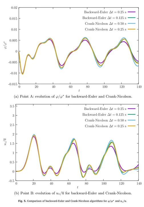
Fig. 5. Comparison of backward-Euler and Crank-Nicolson algorithms for𝜑∕𝜑⋆and u1∕u.

̇n⋆ d+ ∇⋅ [( n⋆_d+1)ud ] =0 (18) where n_d= (1 + n⋆_d)n_d0 (19)

In equation(18)it is assumed that nd0is uniform. For the

Poisson-like equation, after inserting(19), we have, ∇2𝜑 + e 𝜀0 [ ni−ne−nd0 ( 1 + n⋆_d)Zd ] =0 (20)

3. Weak form with distinction of the convective term

Numerical time-integration of equations (5–7) is performed with the backward-Euler method. In 2D, the integrated versions of (5–7) between time-steps t_kand t_k+1(with Δt = t_k+1−t_k) are straightforward: ( n⋆_k+1+1) ( 𝜕u1 𝜕x1 +𝜕u2 𝜕x2 ) +n ⋆ k+1−n⋆k Δt + 𝜕n⋆ k+1 𝜕x1 u₁+𝜕n ⋆ k+1 𝜕x2 u₂=0 (21) ( n⋆_k+1+1) (uk+1−uk Δt ) +(n⋆_k+1+1) ⎧⎪_⎨ ⎪ ⎩ u1𝜕u_𝜕x1 1 +u2𝜕u_𝜕x1 2 u₁𝜕u2 𝜕x1 +u₂𝜕u2 𝜕x2 ⎫ ⎪ ⎬ ⎪ ⎭ || || || || |k+1 + − e(n⋆_k+1+1)Zd md ⎧ ⎪ ⎨ ⎪ ⎩ 𝜕𝜑 𝜕x1 𝜕𝜑 𝜕x2 ⎫ ⎪ ⎬ ⎪ ⎭ || || || ||k+1 +c 2 da nd0 ⎧ ⎪ ⎨ ⎪ ⎩ 𝜕n⋆ 𝜕x1 𝜕n⋆ 𝜕x2 ⎫ ⎪ ⎬ ⎪ ⎭ || || || || |k+1 = { 0 0 } (22) 𝜕2_𝜑 k+1 𝜕x2 1 +𝜕 2_𝜑 k+1 𝜕x2 2 + e 𝜀0 [ ni−ne−nd0 ( 1 + n⋆_k+1)Zd ] =0 (23)

To make use of ﬁnite elements, equations(21–23)are now written in weak form. We introduce the following test functions:

•̃n⋆∈𝒱n(Ω)where𝒱n(Ω) = { ̃n⋆_|̃n⋆_∈_W1,2_{(Ω) ∧}_̃n(Γ n) =0 } •̃u ∈ 𝒱_u(Ω)where𝒱u(Ω) = { ̃u|̃u ∈ W1,2_{(Ω) ∧}_̃u i(Γu) =0 } •̃𝜑 ∈ 𝒱_𝜑(Ω)where𝒱𝜑(Ω) ={̃𝜑|̃𝜑 ∈ W1,2(Ω) ∧̃𝜑(Γ𝜑) =0} where Wm,p(Ω) ={w ∈ Lp(Ω)|D𝜶w ∈ Lp(Ω) ∀|𝜶| ≤ m} (24)

(8)

Fig. 6. Variable width slab: relevant data and results for u1and𝜑. Points A and B indicate monitored u1and𝜑∕𝜑⋆, respectively.

and Lp(Ω)is the space of p−power integrable functions. With this pur-pose, we use the test functions to obtain a weak form of(21–23) inte-grating in the domain Ω,

̃ W = ∫Ω ̃n⋆[(_n⋆ k+1+1 ) 𝜕uj 𝜕xj +n ⋆ k+1−n⋆k Δt + 𝜕n⋆ k+1 𝜕xj uj ] dΩ + ∫Ω ̃u•T ⎡ ⎢ ⎢ ⎢ ⎢ ⎢ ⎣ ( n⋆_k+1+1) (uk+1−uk Δt ) + ( n⋆_k+1+1) ⎧ ⎪ ⎪ ⎨ ⎪ ⎪ ⎩ u1𝜕u_𝜕x1 1 +u2𝜕u_𝜕x1 2 u1𝜕u_𝜕x2 1 +u2𝜕u_𝜕x2 2 ⎫ ⎪ ⎪ ⎬ ⎪ ⎪ ⎭ || || || || || |k+1 ⎤ ⎥ ⎥ ⎥ ⎥ ⎥ ⎦ dΩ + ∫Ω ̃u•T ⎡ ⎢ ⎢ ⎢ ⎢ ⎢ ⎣ − e(n⋆_k+1+1)Zd md ⎧ ⎪ ⎨ ⎪ ⎩ 𝜕𝜑 𝜕x1 𝜕𝜑 𝜕x2 ⎫ ⎪ ⎬ ⎪ ⎭ || || || || |k+1 + ∫Ω c2 da nd0 ⎧ ⎪ ⎪ ⎨ ⎪ ⎪ ⎩ 𝜕n⋆ 𝜕x1 𝜕n⋆ 𝜕x2 ⎫ ⎪ ⎪ ⎬ ⎪ ⎪ ⎭ || || || || || |k+1 ⎤ ⎥ ⎥ ⎥ ⎥ ⎥ ⎦ dΩ + ∫Ω { −∇𝜑_k+1⋅ ∇̃𝜑 + ̃𝜑e 𝜀0 [ ni−ne−nd0 ( 1 + n⋆_k+1)Zd ]} dΩ + ∫Γ_𝜑′̃𝜑 ∇𝜑⏟⏞⏞⏞⏞⏟⏞⏞⏞⏞⏟k+1⋅ v t(t) dΓ_𝜑′=0 (25)

where k and k + 1 are the time-step indices and j is the direction index. This non-symmetry in the test/trial functions was introduced by

(9)

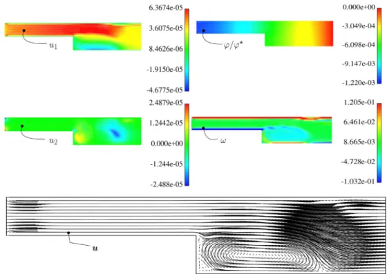
Fig. 7. Variable width slab (t = 500 s): contour plots for u1, u2, 𝜑 and 𝜔. The velocity vectors are also shown.

Brooks and Hughes[20]to ensure stability in the presence of convec-tion. We directly follow Zienkiewicz, et al.[21]in the present applica-tion. The speciﬁc form of the test functioñu• will be detailed later. For the application of the Newton-Raphson method, we require the ﬁrst variation of(25), for which we will make use of the symbol d:

d̃_{W = ∫} Ω ̃n⋆ [ dn⋆_k+1𝜕uj 𝜕xj +(n⋆_k+1+1) 𝜕duj 𝜕xj +dn ⋆ k+1 Δt + 𝜕n⋆ k+1 𝜕xj duj+ 𝜕dn⋆ k+1 𝜕xj uj ] dΩ + ∫Ω ̃u•T ⎡ ⎢ ⎢ ⎢ ⎢ ⎣ ( n⋆_k+1+1 Δt ) duk+1+dn⋆k+1 (_u k+1−uk Δt ) +dn⋆_k+1 ⎧ ⎪ ⎨ ⎪ ⎩ u1𝜕u_𝜕x1 1 +u2𝜕u_𝜕x1 2 u1𝜕u_𝜕x2 1 +u2𝜕u_𝜕x2 2 ⎫ ⎪ ⎬ ⎪ ⎭ || || || || |k+1 ⎤ ⎥ ⎥ ⎥ ⎥ ⎦ dΩ + ∫Ω ̃u•T( n⋆_k+1+1) ⎧⎪_⎨ ⎪ ⎩ du₁𝜕u1 𝜕x1 +du₂𝜕u1 𝜕x2 +u₁𝜕du1 𝜕x1 +u₂𝜕du1 x2 du₁𝜕u2 𝜕x1 +du₂𝜕u2 𝜕x2 +u₁𝜕du2 𝜕x1 +u₂𝜕du2 𝜕x2 ⎫ ⎪ ⎬ ⎪ ⎭ dΩ + ∫Ω ̃u•T ⎡ ⎢ ⎢ ⎢ ⎢ ⎣ − e(n⋆_k+1+1)Zd md ⎧ ⎪ ⎨ ⎪ ⎩ 𝜕d𝜑 𝜕x1 𝜕d𝜑 𝜕x2 ⎫ ⎪ ⎬ ⎪ ⎭ || || || || |k+1 −eZd md dn⋆_k+1 ⎧ ⎪ ⎨ ⎪ ⎩ 𝜕𝜑 𝜕x1 𝜕𝜑 𝜕x2 ⎫ ⎪ ⎬ ⎪ ⎭ || || || || |k+1 + ∫Ω c2 da nd0 ⎧ ⎪ ⎨ ⎪ ⎩ 𝜕dn⋆ 𝜕x1 𝜕dn⋆ 𝜕x2 ⎫ ⎪ ⎬ ⎪ ⎭ || || || || |k+1 ⎤ ⎥ ⎥ ⎥ ⎥ ⎦ dΩ + ∫Ω d̃u•T ⎡ ⎢ ⎢ ⎢ ⎢ ⎣ ( n⋆_k+1+1) (uk+1−uk Δt ) + ( n⋆_k+1+1) ⎧⎪_⎨ ⎪ ⎩ u1𝜕u_𝜕x1 1 +u2𝜕u_𝜕x1 2 u1𝜕u_𝜕x2 1 +u2𝜕u_𝜕x2 2 ⎫ ⎪ ⎬ ⎪ ⎭ || || || || |k+1 ⎤ ⎥ ⎥ ⎥ ⎥ ⎦ dΩ + ∫Ω d̃u•T ⎡ ⎢ ⎢ ⎢ ⎢ ⎣ − e(n⋆_k+1+1)Zd md ⎧ ⎪ ⎨ ⎪ ⎩ 𝜕𝜑 𝜕x1 𝜕𝜑 𝜕x2 ⎫ ⎪ ⎬ ⎪ ⎭ || || || || |k+1 + ∫Ω c2 da nd0 ⎧ ⎪ ⎨ ⎪ ⎩ 𝜕n⋆ 𝜕x1 𝜕n⋆ 𝜕x2 ⎫ ⎪ ⎬ ⎪ ⎭ || || || || |k+1 ⎤ ⎥ ⎥ ⎥ ⎥ ⎦ dΩ + ∫Ω { −∇d𝜑k+1⋅ ∇̃𝜑 + ̃𝜑_𝜀e 0 [ dni d𝜑d𝜑 − dne d𝜑d𝜑 − dn⋆k+1nd0Zd ]} dΩ (26)

We note that, in deriving(26), we made use of the property d̃u = 0. However, note that d̃u•≠ 0. The Newton solution is based on the two deﬁnitions(25–26)using standard techniques (see, e.g. Ref.[22]).

(10)

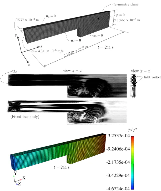
Fig. 8. 3D version of the variable width slab. With the addition of a symmetry plane, boundary conditions are similar to those ofFig. 6, but additional vortices occur at the inlet.

4. Petrov-Galerkin discretization

In terms of discretization, we introduce the interpolations for a given element e. Use is made of the interpolation matrices Ne(𝝃) for udand

𝐍e(𝝃) for scalars n⋆and𝜑, with 𝝃 being the parent-domain coordinates.

Introducing the nodal unknowns (trial functions) for a given element e (ue, n⋆e, and𝜑e), we have the interpolations (for simplicity we omit the

subscript d):

u = Ne(𝝃) ue (27)

n⋆=𝐍_e(𝝃) n⋆_e (28)

̃𝜑 = 𝐍e(𝝃) ̃𝜑e (29)

For the Galerkin projection(25)we require the test functions:

̃u = Ne(𝝃) ̃ue (30) ̃u• =N•_e(𝝃, ue ) ̃ue (31) ̃n⋆₌_𝐍 e(𝝃) ̃n⋆e (32) ̃𝜑 = 𝐍e(𝝃) ̃𝜑e (33)

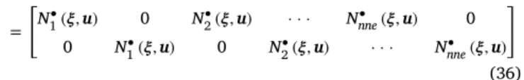
where matrices𝐍e(𝝃), Ne(𝝃) and N•e(𝝃, u) are deﬁned as:

𝐍e(𝝃) = [ N1(𝝃) · · · Nnne(𝝃) ] (34) Ne(𝝃) = [ N1(𝝃) 0 N2(𝝃) · · · Nnne(𝝃) 0 0 N₁(𝝃) 0 N₂(𝝃) · · · N_nne(𝝃) ] (35)

(11)

P. Areias et al. Finite Elements in Analysis and Design 140 (2017) 38–49 N• e(𝝃, u) = [ N•₁(𝝃, u) 0 N•₂(𝝃, u) · · · N•_nne(𝝃, u) 0 0 N• 1(𝝃, u) 0 N • 2(𝝃, u) · · · N • nne(𝝃, u) ] (36) In deﬁnitions(34–36), nne is the number of nodes in each element, here taken as 4 for low-order quadrilateral and 8 for the hexahedron. N• K(𝝃, u) is given by (cf.[21]) N• K(𝝃, u) = NK(𝝃) + 𝛼h 2 u_i ‖u‖𝜕N𝜕xKi (37) where𝛼 is a stabilization parameter, and h is the element characteristic length. The optimal value of𝛼 is given by Ref.[21]:

𝛼 = coth Pe − 1

Pe (38)

where the Péclet number is deﬁned as

Pe =‖u‖ h∕2k (39)

In(39), k is the diffusion constant. Since the diffusion constant, k, is zero in the present case, we have𝛼 = 1. This corresponds to the Stream-ing Upwind Petrov-Galerkin (SUPG)[19,21], specializing the element size from the velocity. The element characteristic length, h, is defined in agreement with Tezduyar and Park[23], as:

h =_∑ 2‖u‖ nne K=1||||𝜕N𝜕XKiui || || (40)

where NKare the shape functions and nne denotes the number of nodes

in each element. We use the isoparametric interpolation[24]. For a low-order quadrilateral we have nne = 4, and the shape functions have the following form:

NK(𝝃) =1₄ ( 1 +𝜉1𝜉1K ) ( 1 +𝜉2𝜉2K ) (41) { 𝜉1K } = {−1, 1, 1, −1} (42) { 𝜉2K } = {−1, −1, 1, 1} (43)

and, for the hexahedron, NK(𝝃) =1₈ ( 1 +𝜉1𝜉1K ) ( 1 +𝜉2𝜉2K ) ( 1 +𝜉3𝜉3K ) (44) { 𝜉1K } = {−1, −1, −1, −1, +1, +1, +1, +1} (45) { 𝜉2K } = {−1, −1, +1, +1, −1, −1, +1, +1} (46) { 𝜉3K } = {−1, +1, −1, +1, −1, +1, −1, +1} (47) 5. Numerical examples

We implemented two speciﬁc ﬁnite elements (quadrilateral and hexahedral) in SimPlas[26]. The ionosphere properties (cf.[25]) are adopted and shown inTable 2. We consider a spherical Al2O3 dust particle with a radius of rd=1 × 10−6 m and𝜌d=3950 Kg/m3. This

agrees with the interval given in Ref.[25]. The ﬁrst example deals with an initial density (and hence charge) imbalance with prescribed𝜑 at the boundary. After this preliminary test, a variable-width slab is presented, where a vortex occurs due to change in section for the 2D case and, in 3D, additional vortices appear at the inlet region. With this example, a complete convergence study is performed.

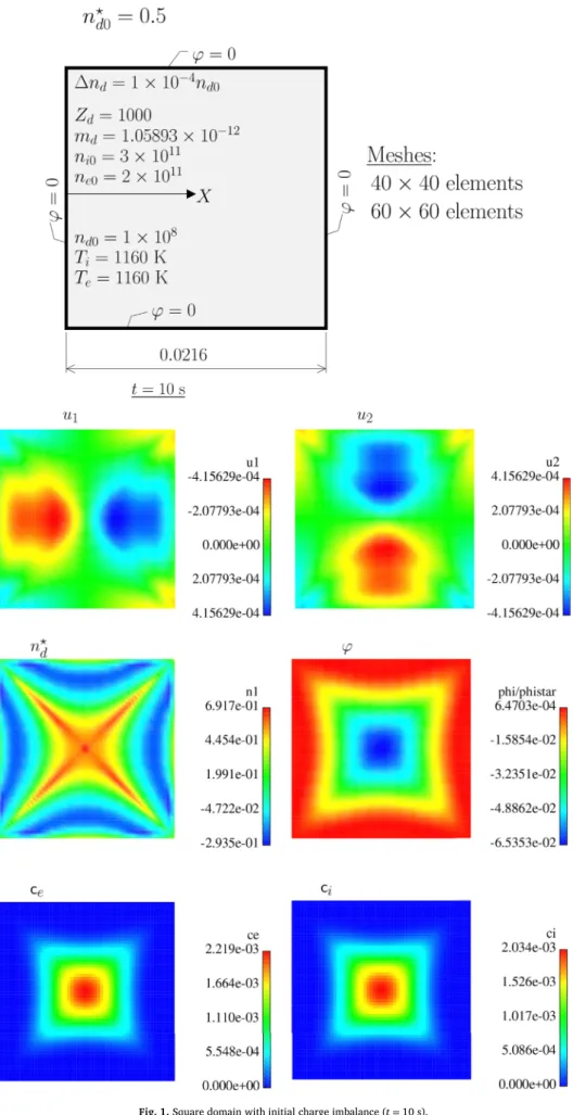
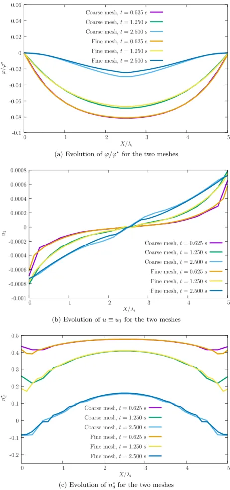
5.1. Square with initial charge imbalance

We now analyze a square plate with initial imbalance of charge. Fig. 1 shows the relevant data, with the charge imbalance being imposed as an initial condition. The goal is to assess the mesh size eﬀect on the results (𝜑∕𝜑⋆_{, u}

d= {u1, u2}and n⋆d). Two meshes are considered:

40 × 40 (coarse) and 60 × 60 (ﬁne) square elements.

Nonlinearity is represented by two parameters, related to deﬁnitions (14–15): 𝖼e= exp(_𝜅e𝜑 BTe ) 1 +_𝜅e𝜑 BTe −1 (48) 𝖼i= exp(− e𝜑 𝜅BTi ) 1 −_𝜅e𝜑 BTi −1 (49)

When the problem is linear,𝖼e=𝖼i=0 and both(48–49)are

subse-quently used in contour plots to assess nonlinearities.Fig. 1shows the contour plots for the aforementioned quantities for t = 10 s. Smooth results are obtained, which are a consequence of the SUPG tech-nique.Fig. 2shows the comparison between the two meshes. It can be observed that results show slight diﬀerences for t = 2.5 s. Nonlinear-ities can be observed inFig. 1where the two parameters𝖼eand𝖼iare

plotted.

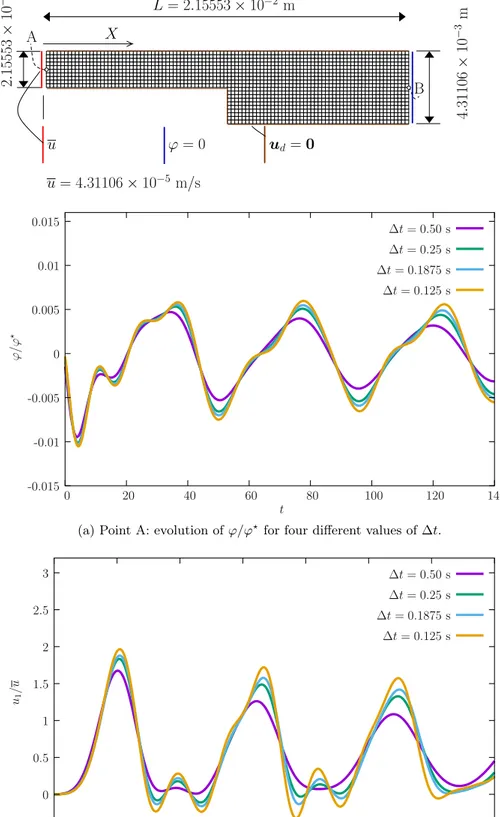
5.2. Vortex in a variable width slab

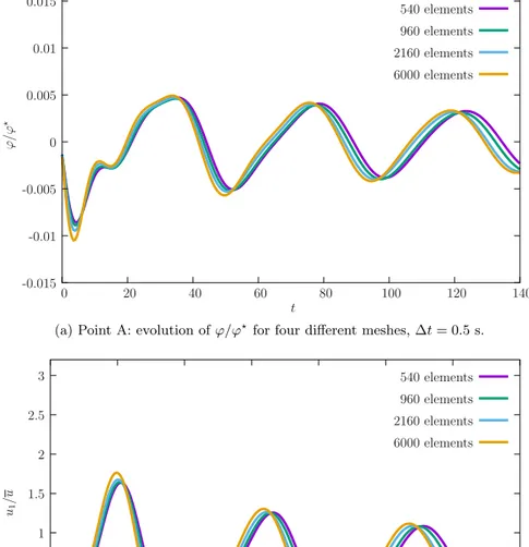
In this test, we introduce slab with a change of section in the direc-tion of ﬂow with the objective of testing the robustness of our com-bination Petrov-Galerkin/Backward Euler integration.Fig. 3shows the dimensions and relevant data for this problem. Time-step sensitivity was found to be very good with the larger time step Δt = 0.5 s provid-ing acceptable detail. In terms of mesh sensitivity, we test 4 meshes, all with square elements. Only slight dependence is observed, cf.Fig. 6. Contour plots for u1, u2,𝜑 and 𝜔 are shown inFig. 7. We can observe the smooth behavior of all quantities.

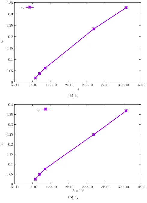
We use a very ﬁne mesh with 13500 elements as a reference solution to assess the mesh convergence of u1∕u and𝜑∕𝜑⋆. Errors are deﬁned using the uniform norm as:

eu= ‖u1∕u − uref∕u‖∞,[0,140] ‖uref∕u‖∞,[0,140] (50) e_𝜑= ‖𝜑∕𝜑 ⋆₋_𝜑 ref∕𝜑⋆‖∞,[0,140] ‖𝜑ref∕𝜑⋆‖∞,[0,140] (51) where the interval t ∈ [0, 140] s is used.Fig. 4shows euand e𝜑as

func-tions of h where h is the edge size of the square elements. We use 5 dif-ferent values of h to assess convergence: h = 3.59241 × 10−4_{, 2.69441 ×} 10−4, 1.34721 × 10−4, 1.19761 × 10−4, 1.07777 × 10−4. We conclude that linear convergence occurs with this formulation.

Alternative time-integration algorithms exist for the ﬂuid equations, one of the most popular is the Crank-Nicolson algorithm[27], which combines fully backward-Euler and forward-Euler terms to obtain second-order convergence. We found that it allows larger time-steps, at the cost of more function evaluations, seeFig. 5. Therefore, for rel-atively inexpensive function evaluations, the Crank-Nicolson algorithm is preferable.

The 3D version of the slab is shown inFig. 8, where the boundary conditions are equivalent to those inFig. 3, but with the zero velocity around the external boundary, except in the symmetry plane, in which u3=0.Fig. 8shows another type of vortex, which was found in the inlet section, with a rotation axis parallel to x. The vortex after the jump is also shown in this Figure and is similar to what was found in the 2D example. In the view z − z we can see the variation of the vortex shape at the jump along the thickness (the front face alone is shown below).

(12)

6. Conclusions

We introduced a new formulation for dust-acoustic waves in unmag-netized plasma. This consists of a Petrov-Galerkin finite element com-bined with the backward-Euler time integration method. Nonlinear effects are included in the number density of ions and electrons, which are affected exponentially by the electrostatic potential. Numerical experiments showed very good robustness with respect to mesh size and time-step size and absence of instabilities. Waves resulting from the nonlinear constitutive laws for number densities are sharply observed. As a follow-up contribution, we will include viscosity (less important than in classical plasma analysis, cf.[11]) and will introduce the mag-netic field, along with a specialized version of Maxwell’s equations. References

[1] I. Langmuir, Oscillations in ionized gases, Proc. Natl. Acad. Sci. 14 (August 1928) 627–637.

[2] F.F. Chen, Introduction to Plasma Physics and Controlled Fusion, 2 edition, Plasma Physics, vol. 1, Plenum Press, New York, 1984.

[3] P.K. Shukla, A.A. Mamun, Introduction to Dusty Plasma Physics. Series in Plasma Physics, IOP Institute of Physics Publishing, 2002.

[4] C.K. Goertz, G. Morﬁll, A model for the formation of spokes in Saturn’s ring, Icarus 53 (1983) 219–229.

[5] M. Horanyi, H.L.F. Houpis, D.A. Mendis, Charged dust in the earth’s magnetosphere, Astrophys. Space Sci. 144 (1–2) (1988) 215–229.

[6] O. Havnes, C.K. Goertz, G.E. Morﬁll, E. Grün, W. Ip, Dust charges, cloud potential, and instabilities in a dust cloud embedded in a plasma, J. Geophys. Res. 92 (A3) (1987) 2281–2287.

[7] N.N. Rao, P.K. Shukla, M.Y. Yu, Dust-acoustic waves in dusty plasmas, Planet Space Sci. 38 (4) (1990) 543–546.

[8] F.G. Verheest, General dispersion relations for linear waves in multicomponent plasmas, Physica 34 (1967) 17–35.

[9] A.A. Mamun, P.K. Shukla, Electrostatic solitary and shock structures in dusty plasmas, Phys. Scr. 98 (2002) 107–114.

[10]A. Barkan, R.L. Merlino, N. D’Angelo, Laboratory observation of dust-acoustic wave mode, Phys. Plasmas 2 (10) (1995) 3563–3565.

[11] R. Merlino, J. Goree, Dusty plasmas in the laboratory, industry, and space, Phys. Today 57 (7) (2004) 32–38.

[12] C. Sovinec, A. Glasser, T. Gianakon, D. Barnes, R. Nebel, S. Kruger, D. Schnack, S. Plimpton, A. Tarditi, M. Chu, Nonlinear magnetohydrodynamics simulation using high-order ﬁnite elements, J. Comput. Phys. 195 (1) (2004) 355–386. [13] C.R. Sovinec, J.R. King, Analysis of a mixed semi-implicit/implicit algorithm for

low-frequency two-ﬂuid plasma modeling, J. Comput. Phys. 229 (2010) 5803–5819.

[14] S.C. Jardin, J. Breslau, N. Ferraro, A high-order implicit ﬁnite element method for integrating the two-ﬂuid magnetohydrodynamic, J. Comput. Phys. 226 (2007) 2146–2174.

[15] R. Codina, N. Hernández-Silva, Stabilized ﬁnite element approximation magneto-hydrodynamics equations, Comput. Mech. 38 (2006) 344–355. [16] J.N. Shadid, R.P. Pawlowski, E.C. Cyr, R.S. Tuminaro, L. Chacón, Scalable implicit

incompressible resistive MHD with stabilized FE and fully-coupled Newton-Krylov-AMG, Comp. Method Appl. M. 304 (2016) 1–25.

[17] B. Srinivasan, A. Hakim, U. Shumlak, Numerical methods for two-ﬂuid dispersive fast MHD phenomena, Commun. Comput. Phys. 10 (1) (2011) 183–215. [18] D. Levy, C.-W. Shu, J. Yan, Local discontinuous galerkin methods for nonlinear

dispersive equations, J. Comput. Phys. 196 (2004) 751–772.

[19] T.J.R. Hughes, A.N. Brooks, A multi-dimensional upwind scheme with no cross wind diﬀusion, in: T.J.R. Hughes (Ed.), Finite Elements for Convection Dominated Flows, Number 34, ASME, AMD, New York, 1979.

[20] A.N. Brooks, T.J.R. Hughes, Streamline upwind/Petrov-Galerkin formulations for convection dominated ﬂows with particular emphasis on the incompressible Navier-Stokes equations, Comp. Method Appl. M. 32 (1982) 199–259.

[21] O.C. Zienkiewicz, R.L. Taylor, P. Nithiarasu, 7 edition, The Finite Element Method for Fluid Dynamics, vol. 3, Butterworth-Heinemann, Elsevier, 2014.

[22] K.-J. Bathe, Finite Element Procedures, Prentice-Hall, Englewood Cliﬀs, 1996. [23] T.E. Tezduyar, Y.J. Park, Discontinuity capturing ﬁnite element formulations for

nonlinear convection-diﬀusion-reaction problems, Comp. Method Appl. M. 59 (1986) 307–325.

[24] T.J.R. Hughes, The Finite Element Method, Linear Static and Dynamic Finite Element Analyses, Prentice-Hall, Englewood Cliﬀs, N.J, 1987.

[25] H. Fu, W.A. Scales, Model for charged dust expansion, Phys. Plasmas 20 (073704) (2013).

[26] P. Areias. Simplas.http://www.simplas-software.com.

[27] J. Crank, P. Nicolson, A practical method for numerical evaluation of solutions of partial diﬀerential equations of the heat-conduction type, Adv. Comput. Math. 6 (207–226) (1996) Reprinted from Proc Camb Phil Soc 43 (1947) 50–67.