Modelling daily and annual cycles of temperature in two types of soil

Texto

(1)Symposium no. 04. Paper no. 1820. Presentation: poster. Modelling daily and annual cycles of temperature in two types of soil ANDRADE J.A. and ABREU F.G. Departamento de Geociências, Universidade de Évora, Évora,Ciências do Ambiente, Instituto Superior de Agronomia, Lisboa, Portugal Abstract Soil temperature influences strongly crop development and growth. The daily and annual periodic variations of soil temperature follow closely the time-course of solar irradiance. The temperature profiles of a Luvisol and a Vertisol, in the Mediterranean region of southern Portugal, were measured at six depths (2 to 32 cm), and the analysis of daily and annual temperature cycles was performed by means of Fourier series; daily cycles were studied based on data from four typical clear days through the year. Daily course of soil temperature was well described by the two first Fourier harmonics, while the annual course of soil temperature was described satisfactorily by the first harmonic alone, which explain more than 90% of total variance. Soil heterogeneity effects on the simulation and on thermal wave damping are also discussed. Keywords: soil temperature simulation, Fourier series, damping depth Introduction Prediction of soil temperature is important for crop growth and development. Soil temperature depends both on the soil surface energy balance as on thermal properties of the soil (de Vries, 1975; Buchan, 1982). Daily and annual soil temperature variations are periodic in response to the time-course of solar radiation at the soil-atmosphere interface. The thermal properties of the soil (conductivity, diffusivity and heat capacity) govern the penetration of the daily and annual temperature waves into the soil (Monteith and Unsworth, 1990). Several authors have used a single harmonic or a superposition of a finite number of Fourier harmonics to describe the daily and annual cycling of soil temperature (Krishman and Kushwaha, 1972; Ghuman and Lal, 1982; Andrade et al., 1993). However, the applicability of this analytical solution is difficult (Krishman and Kushwaha, 1972; Gupta et al., 1984; Massman, 1992), because soil thermal properties vary with depth, namely the thermal diffusivity (Campbell, 1987). The objective of this work is to evaluate the simulation of the time course of soil temperature through daily and annual cycles in two types of soil at six depths (2, 4, 6, 8, 16 and 32 cm) using Fourier series and to discuss the influences of soil profile heterogeneity on the thermal wave damping with depth.. 1820-1.

(2) 17th WCSS, 14-21 August 2002, Thailand. ANDRADE & ABREU. Materials and Methods Theory Daily or annual temperature variation at any depth z in an homogenous and isotropic layer of a soil (thermal diffusivity is constant with depth and time) can be represented by Fourier series as ∞. T ( z , t ) = Tave + ∑ Cz , n ( sin nωt + φn - zn 1/2 D). (1). n =1. where Tave (ºC) is the average temperature in the layer, T(z,t) is the soil temperature at depth z and time t, in ºC, n is the nth harmonic (n = 1 is the first harmonic corresponding to the single sinusoidal representation), ω is the angular frequency of the oscillation given by 2π/P (P is the daily or annual period of the oscillation), Cz,n is the semi-amplitude (Tmax - Tave or Tave - Tmin) of the harmonic n and at depth z, and φn is the phase angle of the nth harmonic (Krishman and Kushwaha, 1972; Ghuman and Lal, 1982). Cz,n decreases exponentially with depth as: C z , n = C 0, n exp (− z / Dn) (2) where C0,n is the semi-amplitude at soil surface and Dn, is the damping depth of the nth harmonic. D is the damping depth of the first harmonic. The depth penetration of T is the sum of the penetrations of each harmonic. The number of harmonics required for a good description of the temperature (Equation 1) must explain a high percentage of %Variance =. (Cn 2 / 2) × 100 ST 2. (n = 1,...,3) (3). %Variance = Cn /ST × 100 2. 2. (n = 4). the total variance (ST2) of temperature data about Tave. According to Panofsky and Brier (1958), the fraction of total variance accounted for by each of the first four harmonics is. Procedures The field experiments were located in Monte dos Álamos, Évora (lat.: 38º30′N; long. 7º45′W) and in Tapada da Ajuda, Lisboa (lat.: 38º42′N; long. 9º11′W). The soils were a Luvisol (Évora) and a Vertisol (Lisboa). The former is loamy-sand textured, with a bulk density ranging from 1.48 in the upper layer (0-20 cm depth) to 1.67 g cm-3 in the lower layer and with an organic matter content less than 1%. The Vertisol is loam-clay textured, with a bulk density ranging from 1.22 in the upper layer (0 - 15 cm depth) and 1.33 g cm-3 in the lower layer and with an organic matter content less than 3%. The soil water content at 15 atm ranges from 0.10 cm3 cm-3 in the upper layer to 0.23 cm3 cm-3 in the lower layer of the Luvisol and from 0.26 cm3 cm-3 to 0.35 cm3 cm-3 in the Vertisol; the water content at 1/3 atm ranges from 0.23 cm3 cm-3 to 0.35 cm3 cm-3 in the Luvisol and from 0.42 cm3 cm-3 to 0.43 cm3 cm-3 in the Vertisol. In both soils, temperature profiles were measured with copper-constantan (Type T) thermocouples at 2, 4, 6, 8, 16 and 32-cm depth and a CR 10 data logger (Campbell Scientific, Inc.). Average temperatures were recorded hourly, daily and for 10-day periods.. 1820-2.

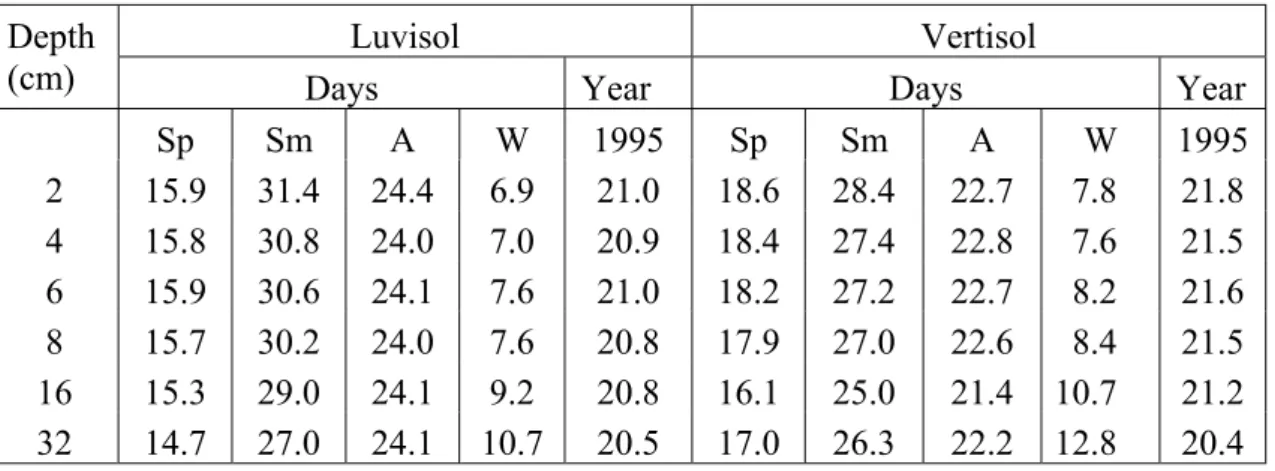
(3) 17th WCSS, 14-21 August 2002, Thailand. ANDRADE & ABREU. Daily courses of soil temperature at each depth were simulated for 4 clear sky days through the fitting of the first 4 harmonics of the Equation (1) to the measured hourly averaged temperature values. Two days are close to summer (day Sm) and winter (day W) solstices and two days are close to vernal (day Sp) and autumnal (day A) equinoxes. Vertisol water content was high on days W (0.38 cm3 cm-3) and Sp (0.39 cm3 cm-3), low on day Sm (0.24 cm3 cm-3) and medium on day A (0.30 cm3 cm-3); Luvisol water content was low on days A (0.09 cm3 cm-3) and Sm (0.14 cm3 cm-3) and medium on days Sp (0.19 cm3 cm-3) and W (0.22 cm3 cm-3). The annual course of soil temperature was simulated for 1995 through the fitting of Equation (1) and using the decade as the time unit. Annual precipitation was 669 mm in Tapada da Ajuda (731 mm in the normal year) and 664 mm in Monte dos Álamos (normal year = 665 mm). Cn and the percentage of total variance explained by each harmonic were estimated for each depth and the damping depth was calculated from measured amplitudes and from amplitudes simulated by the first two harmonics. Results and Discussion Mean temperature was nearly constant along both soil profiles on days Sp and A and in 1995, but it decreased more than 3ºC with depth on day Sm and it increased more than 3,5ºC on day W (Table 1). In the Vertisol, daily mean temperatures at 32-cm depth were always greater than at 16-cm depth. For the whole profile, mean temperatures on days Sp, Sm, A and W were, respectively, 15.5±0.5ºC, 29.8±1.6ºC, 24.1±0.1ºC and 8.2± 1.5ºC in the Luvisol and 17.7±1.0ºC, 26.9±1.2ºC, 22.4±0.6ºC, 9.3±2.1ºC in the Vertisol. Mean temperatures during 1995 was 20.8±0.2ºC in the Luvisol and 21.3±0.5ºC in the Vertisol. Table 1 Mean temperatures (ºC) measured at several depths, for days Sp, Sm, A and W, and for 1995 in the Luvisol and the Vertisol. Depth (cm) 2 4 6 8 16 32. Sp 15.9 15.8 15.9 15.7 15.3 14.7. Luvisol Days Sm A 31.4 24.4 30.8 24.0 30.6 24.1 30.2 24.0 29.0 24.1 27.0 24.1. W 6.9 7.0 7.6 7.6 9.2 10.7. Year 1995 21.0 20.9 21.0 20.8 20.8 20.5. Sp 18.6 18.4 18.2 17.9 16.1 17.0. Vertisol Days Sm A 28.4 22.7 27.4 22.8 27.2 22.7 27.0 22.6 25.0 21.4 26.3 22.2. W 7.8 7.6 8.2 8.4 10.7 12.8. Year 1995 21.8 21.5 21.6 21.5 21.2 20.4. Daily cycles Measured and simulated hourly soil temperatures on day Sp, at 2-cm, 16-cm and 32-cm depth, are illustrated in Figure 1. The measured daily courses of temperature were nearly harmonic between 2 and 16-cm in the Luvisol and between 2 and 8-cm in the Vertisol. The use of the first harmonic alone was not adequate to describe thermal variation, mainly because maximum temperatures were underestimated and warming periods (always equal to 12 hours) were overestimated. Temperature variation at 4-cm,. 1820-3.

(4) 1. 1. 1. 3. 3. 3. 5. 5. 5. 9. 11 13 15 Time (hours). 7. 9. 11 13 15 Time (hours). 9. 11 13 15 Time (hours). Luvisol (32 cm depth). 7. Luvisol (16 cm depth). 7. Luvisol (2 cm depth). 17. 17. 17. 19. 19. 19. 21. 21. 21. 23. 23. 23. 13. 14. 15. 16. 18 17. 19. 19 18 17 16 15 14 13 12. 5. 10. 15. 20. 25. 30. 1. 1. 1. 3. 3. 3. 5. 5. 5. 7. 7. 7. 11 13 15 Time (hours). 11 13 15 Time (hours). 9. 13. 15 Time (hours). 11. Vertisol (32cm depth). 9. Vertisol (16cm depth). 9. Vertisol (2cm depth). 17th WCSS, 14-21 August 2002, Thailand. 17. 17. 17. 19. 19. 19. 21. 21. 21. 23. 23. 23. 1820-4. Figure 1 Daily (day Sp) soil temperatures at 2 cm, 16 cm and 32 cm depth measured (X) and simulated with the first harmonic (___), the first two harmonics (---) three harmonics (_ _ _) and four harmonics (_-_-) in the Luvisol and the Vertisol.. 13. 14. 15. 16. 17. 18. 19. 12. 14. 16. 18. 5. 10. 15. 20. 25. 30. ANDRADE & ABREU. Soil temperature (ºC). Soil temperature (ºC). Soil temperature (ºC). Soil temperature (ºC) Soil temperature (ºC) Soil temperature (ºC).

(5) ANDRADE & ABREU. 17th WCSS, 14-21 August 2002, Thailand. 6-cm and 8-cm depth and on days Sm, A and W are not shown because they were similar to those obtained at 2-cm depth and on day Sp, respectively. Table 2 shows the total variance of the soil temperatures around its daily average and the percentage accounted for by different harmonics at six depths in both soils. The superposition of the two first harmonics improved the adjustment in comparison to the first harmonic alone and explained generally more than 98% of total variance, until 16cm depth in the Luvisol and until 8-cm depth in the Vertisol, making unnecessary the use of the 3rd and 4th harmonics. However, the relative contribution of the first harmonic increased generally with soil depth and with day length (Table 2). These results show that the daily course of soil temperature is well described by the two first harmonics, for clear days along the year. Two harmonics were also sufficient to describe thermal course in the upper 30-cm in a silty-loam soil studied by Gupta et al. (1984) and at 5-cm depth in a sandy loam soil studied by Ghuman and Lal (1982). The real size of the warming period (WP) is generally less than 12 hours (Table 3) and it seems to be the main factor of the asymmetries in relation to the sinusoidal model (1st harmonic). The superposition of the two first harmonics reduced the durations of the simulated warming periods, approaching them to those measured. The increase of WP with day length helps to explain the high percentages of total variance accounted for by the first harmonic in long days. At 16-cm depth in the Vertisol and at 32-cm depth in both soils the harmonic behaviour of temperature course was not as evident as it was at the upper layers (Figure 1), and the relative contribution of the first harmonic was more variable and generally smaller than close to the surface. Changes in thermal behaviour may be associated to changes in soil properties with depth. In addition, the sensitivity of the thermocouples might explain the results at 32-cm depth because thermal amplitudes were very small. The damping with depth of the daily temperature wave was visible (Figure 1) both in the reduction of amplitude as in the delay of occurrence of thermal extremes. At 2-cm depth in the Luvisol, the amplitudes reached 30ºC on day Sm and 14ºC on day W; in the Vertisol they reached 29ºC on day Sm and Sp and 5ºC on day W. At 32-cm depth, daily thermal amplitudes were around 2ºC. Thermal maximum at 2-cm depth occurred at 1516 hours and 2-3 hours later at 16 cm depth in the Luvisol or 1 hour later at 8 cm depth at the Vertisol. Thermal extremes were out of phase at 16-cm depth in the Vertisol and at 32-cm depth in the Luvisol. Damping depth was calculated for two thermal profiles in each soil because the thermal behaviour of the soils was not constant along each profile: Profile 1 (P1) includes temperatures measured in both soils at 2, 4, 6, 8, 16 and 32 cm depth while P2 includes measurements of temperature from 2 cm to 16 cm depth in the Luvisol and from 2 cm to 8 cm depth in the Vertisol. D values estimated in both soils (from measured or simulated amplitudes) for the full profiles (P1) were greater than those estimated for profiles P2 (Table 4), i.e., the velocity of the thermal wave was smaller in P2 than in subjacent layers. On the other hand, the differences in D between P1 and P2 were larger in the Vertisol than in the Luvisol. In the Luvisol, D estimated from measured temperatures ranged from 11.1 cm (day Sm) to 14.3 cm (day W) for the full profile and from 10.6 cm (day Sp) to 12.1 (day W) for P2; in the Vertisol, D values ranged from 12.2 cm (day Sm) to 19.6 cm (day W) for P1 and from 8.7 cm (day Sm) to 15.9 cm (day W) for P2.. 1820-5.

(6) 17th WCSS, 14-21 August 2002, Thailand. 59.7 35.2 19.4 13.6 1.9 0.3. 13.6 11.3 5.4 4.2 0.3 1.5. 4.2 6.5 3.7 2.7 0.5 0.3. 69.5 68.4 66.3 63.8 57.7 48.2. 2 4 6 8 16 32. 2 4 6 8 16 32. 2 4 6 8 16 32. 2 4 6 8 16 32. Day A. Day W. Year 1995. Day Sm. Day Sp. 40.2 27.2 20.7 15.3 1.5 1.0. 2 4 6 8 16 32. Variance. (oC). Depth. (cm). DAY/YEAR. 0.1 0.1 0.1 0.1 0.4 13.3 0.3 0.3 0.3 0.3 0.3 0.7. 4.2 3.7 3.1 2.6 1.3 1.9 9.8 9.1 7.9 6.7 3.8 5.5 36.8 37.6 37.5 38.2 38.7 52.7 0.6 0.7 0.7 0.8 0.4 0.5. 95.7 96.2 96.7 97.2 98.0 82.3. 89.6 90.4 91.6 92.9 95.7 89.9 60.7 59.6 59.4 58.1 50.0 30.6 92.0 90.2 92.5 92.7 93.2 94.9. 0.3 0.6 0.2 0.2 0.1 0.1. 0.5 0.5 0.6 0.9 4.1 2.8. 0.3 0.2 0.1 0.1 0.4 6.3. 10.5 9.7 8.7 7.5 2.0 46.1. 89.0 89.9 91.0 92.2 96.8 33.5. 3. 2. 1. 0.5 1.6 0.5 0.5 0.6 0.5. 0.4 0.6 0.6 0.7 1.5 2.7. 0.3 0.2 0.2 0.1 0.1 2.2. 0.1 0.1 0.0 0.0 0.0 0.3. 0.1 0.1 0.1 0.1 0.3 5.0. 4. 93.3 93.2 94.0 94.2 94.2 96.0. 98.4 98.2 98.1 97.9 94.4 88.9. 99.9 99.9 100.0 100.0 99.9 98.3. 100.0 100.0 99.9 99.9 99.8 97.9. 99.9 99.9 99.9 99.9 99.5 90.9. 1+...+4. 1820-6. 92.6 90.9 93.2 93.5 93.5 95.4. 97.5 97.1 96.9 96.3 88.8 83.4. 99.4 99.5 99.5 99.6 99.5 95.4. 99.8 99.8 99.8 99.8 99.3 84.3. 99.5 99.6 99.7 99.7 98.8 79.6. 1+ 2. % of variance accounted for by harmonic of n order. Luvisol. 52.3 47.4 44.2 44.4 35.2 26.5. 4.2 6.5 3.7 2.7 0.5 0.3. 13.6 11.3 5.4 4.2 0.3 1.5. 59.7 35.2 19.4 13.6 1.9 0.3. 40.2 27.2 20.7 15.3 1.5 1.0. (oC). Variance. 91.1 90.8 92.1 92.1 93.6 95.3. 78.0 77.3 79.3 78.6 91.2 74.3. 85.8 85.4 87.1 87.0 46.4 75.1. 94.4 94.4 95.7 96.4 82.0 50.0. 90.8 90.4 92.2 93.2 76.5 88.1. 1. 0.6 0.7 0.4 0.5 0.7 0.7. 20.4 20.7 19.1 19.6 0.8 19.8. 13.4 13.7 12.0 11.9 37.3 20.2. 5.3 5.4 3.9 3.1 12.1 23.7. 7.9 7.9 6.6 5.6 18.9 5.3. 2. 0.1 0.1 0.0 0.0 0.0 0.0. 0.6 1.4 0.8 1.0 3.3 1.8. 0.6 0.7 0.4 0.4 0.3 0.1. 0.2 0.2 0.2 0.3 4.5 17.7. 1.0 1.4 0.8 0.6 1.8 0.7. 3. 0.6 0.7 0.7 0.7 0.6 0.5. 0.3 0.4 0.2 0.3 1.1 0.7. 0.1 0.1 0.4 0.6 13.8 3.9. 0.0 0.0 0.1 0.1 0.5 4.2. 0.2 0.1 0.2 0.3 1.8 4.2. 4. 91.7 91.5 92.5 92.6 94.3 95.9. 98.3 97.9 98.5 98.2 92.0 94.1. 99.2 99.1 99.1 98.9 83.7 95.3. 99.7 99.8 99.6 99.5 94.1 73.6. 98.7 98.3 98.8 98.9 95.4 93.4. 1+2. 92.4 92.3 93.2 93.4 94.9 96.5. 99.3 99.7 99.5 99.4 96.3 96.6. 99.9 99.9 99.9 99.9 97.8 99.4. 100.0 100.0 99.9 99.9 99.1 95.5. 99.8 99.8 99.8 99.8 99.0 98.3. 1+...+4. Vertisol % of variance accounted for by harmonic of n order. Table 2 Total variance (ºC) of the soil temperatures at various depths in the Luvisol and the Vertisol and the percentage accounted for by the four first harmonics on day Sp, Sm, A and W and on year 1995.. ANDRADE & ABREU.

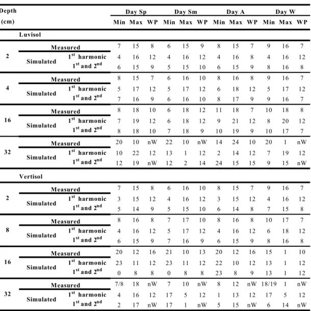
(7) 17th WCSS, 14-21 August 2002, Thailand. ANDRADE & ABREU. Table 3 Measured and simulated temperature extremes (Max, Min, inºC) and warming periods (WP, in hours), at 2, 4, 16 and 32 cm depth in the Luvisol and in the Vertisol, for daily cycles. NW-more than one Warming period. Depth. Day Sp. (cm). Day Sm. Day A. Day W. Min Max WP Min Max WP Min Max WP Min Max WP Luvisol. 2. 4. 16. 32. Measured 1 st harmonic Simulated 1 st and 2nd. 7. 15. 8. Measured 1 st harmonic Simulated 1 st and 2nd. 8. Measured 1 st harmonic Simulated 1 st and 2nd Measured 1 st harmonic Simulated 1 st and 2nd. 6. 15. 9. 8. 15. 7. 9. 16. 7. 4. 16. 12. 4. 16. 12. 4. 16. 8. 6. 15. 9. 5. 15. 10. 6. 15. 9. 4. 16. 12. 8. 16. 15. 7. 6. 16. 10. 8. 16. 8. 9. 8. 16. 7. 5. 17. 12. 5. 17. 12. 6. 18. 12. 7. 16. 9. 6. 16. 10. 8. 17. 9. 5. 17. 12. 9. 16. 7. 8. 18. 10. 6. 18. 12. 11. 18. 7. 10. 18. 8. 7. 19. 12. 6. 18. 12. 9. 21. 12. 8. 20. 12. 8. 18. 10. 7. 18. 9. 10. 19. 9. 10. 17. 7. 20. 10. nW. 22. 10. nW. 14. 24. 10. 20. 1. nW. 10. 22. 12. 13. 1. 12. 2. 14. 12. 7. 19. 12. 12. 19. nW. 12. 2. 14. 24. 15. 15. 9. 15. nW. Measured 1 st harmonic Simulated 1 st and 2nd. 7. 15. 8. 6. 16. 10. 8. 15. 7. 9. 16. 7. 3. 15. 12. 4. 16. 12. 3. 15. 12. 4. 16. 12. 5. 14. 9. 5. 15. 10. 6. 14. 8. 7. 15. 8. Measured 1 st harmonic Simulated 1 st and 2nd. 8. 16. 8. 7. 17. 10. 8. 16. 8. 10. 17. 7. 4. 16. 12. 5. 17. 12. 4. 16. 12. 6. 18. 12. 6. 15. 9. 7. 16. 9. 6. 15. 9. 8. 16. 8. Measured 1 st harmonic Simulated 1 st and 2nd. 20. 12. 16. 21. 10. 13. 20. 12. 16. 15. 1. 10. 23. 11. 12. 23. 11. 12. 22. 10. 12. 13. 1. 12. 0. 8. 8. 0. 8. 8. 23. 8. 9. 13. 1. 12. Measured 1 st harmonic Simulated 1 st and 2nd. 7/8. 18. nW. 7. 10. nW. 8. 12. nW 18/19. 1. nW. 4. 16. 12. 17. 5. 12. 1. 13. 12. 17. 5. 12. 2. 17. nW. 17. 1. nW. 5. 15. nW. 6. 14. nW. Vertisol 2. 8. 16. 32. These results show that the simulation of soil temperature with Fourier series can be applied to an homogeneous layer of soil. In this case, temperatures at any depth within the layer can be obtained from temperatures measured at any other depth if the D (or the thermal diffusivity) is known for the layer (Horton and Wierenga, 1983). Annual cycles The annual variation of soil temperature was nearly harmonic at any depth in both soils (Figure 2). The first harmonic alone explained more than 90% of the total variance of soil temperature at any depth (Table 2) and its contribution increased slightly from 4cm depth to 32-cm depth in both soils (ranging from 90.2% to 94.9% in the Luvisol and from 90.8% to 95.3% in the Vertisol). The contributions of higher orders of harmonics were very small. Most of the non-periodic variations in Figure 2 were associated to changes of soil water content due to irregular rainfall and high evaporation rates, which. 1820-7.

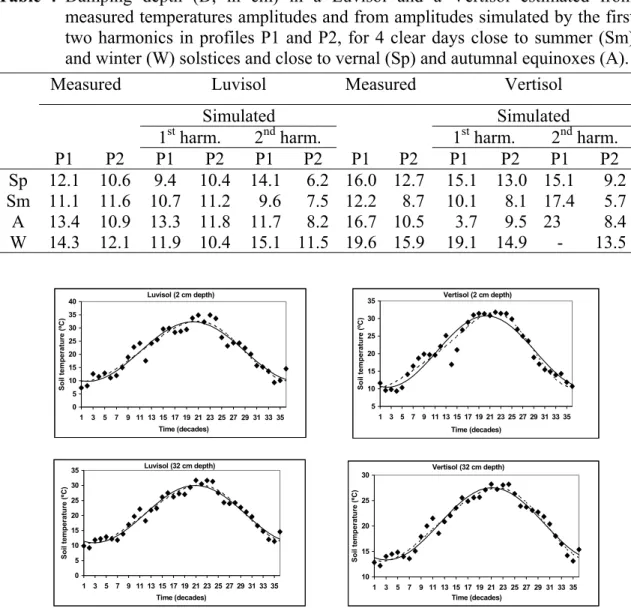
(8) 17th WCSS, 14-21 August 2002, Thailand. ANDRADE & ABREU. are typical of Mediterranean climate. The amplitudes of these irregularities are small and they are not well described by the 2nd, 3rd and 4th harmonics, but only by harmonics of higher order. Table 4 Damping depth (D, in cm) in a Luvisol and a Vertisol estimated from measured temperatures amplitudes and from amplitudes simulated by the first two harmonics in profiles P1 and P2, for 4 clear days close to summer (Sm) and winter (W) solstices and close to vernal (Sp) and autumnal equinoxes (A). Measured Luvisol Measured Vertisol. Sp Sm A W. P1 12.1 11.1 13.4 14.3. P2 10.6 11.6 10.9 12.1. P1 P2 16.0 12.7 12.2 8.7 16.7 10.5 19.6 15.9. Luvisol (2 cm depth). 40 35 30 25 20 15 10 5. 30 25 20 15 10 5. 0 1. 3. 5. 7. 1 3 5 7 9 11 13 15 17 19 21 23 25 27 29 31 33 35. 9 11 13 15 17 19 21 23 25 27 29 31 33 35 Time (decades). Time (decades). Luvisol (32 cm depth). Vertisol (32 cm depth). 30. 30 Soil temperature (ºC). Soil temperature (ºC). 35. Simulated 1st harm. 2nd harm. P1 P2 P1 P2 15.1 13.0 15.1 9.2 10.1 8.1 17.4 5.7 3.7 9.5 23 8.4 19.1 14.9 13.5 Vertisol (2 cm depth). 35 Soil temperature (ºC). Soil temperature (ºC). Simulated 1st harm. 2nd harm. P1 P2 P1 P2 9.4 10.4 14.1 6.2 10.7 11.2 9.6 7.5 13.3 11.8 11.7 8.2 11.9 10.4 15.1 11.5. 25 20 15 10 5 0. 25 20 15 10. 1 3 5 7 9 11 13 15 17 19 21 23 25 27 29 31 33 35. 1. Time (decades). 3. 5. 7. 9 11 13 15 17 19 21 23 25 27 29 31 33 35 Time (decades). Figure 2 Annual (1995) soil temperatures at 2 cm and 32 cm depth, measured (X) and simulated with the first harmonic (___), and the two first harmonics (---), in the Luvisol and the Vertisol. The number of harmonics required for simulation of annual cycles of soil temperature seems to depend mainly on the climate conditions of the region. For example, Khrishnan and Kushwaha (1972) need two harmonics to describe the annual course of soil temperature between 10-cm and 120-cm depth in a region of India (affected by Southwest monsoons) and had to include the third harmonic for upper layers.. 1820-8.

(9) ANDRADE & ABREU. 17th WCSS, 14-21 August 2002, Thailand. Carson (1963) reported that 93.0-99.8% of the total variance was explained by the first harmonic in a humid region (Argonne, USA) where annual rainfall and soil water content variations are not as irregular as in Mediterranean areas. Figureueiredo and Gonçalves (1991) described the annual variation of soil temperature in Bragança, North Portugal, with the first harmonic alone, which explained between 89% and 90% of the total variance. Furthermore, data configureuration (weekly, decades or mensal data) may influence the frequency and the amplitude of the non-periodic fluctuations of climatic elements and thus, the contribution of each harmonic for the total variance around average temperature. Thermal amplitudes in the annual cycle decreased exponentially with depth but this decrease was smaller than in the daily cycle, i.e., damping depth annual values were higher than daily values. Furthermore, annual values of D were higher in the Luvisol (170 cm) than in the Vertisol (100 cm). Conclusions 1) Daily course of soil temperature is well described by the first two Fourier harmonics, for clear days through the year. The fraction of total variance accounted for by the first harmonic increased with day length. 2) Annual course of soil temperature is described satisfactorily by the first harmonic alone. Non-periodic fluctuations due to concentrated and irregular rain are not well-describe by the 2nd, 3rd and 4th harmonics. 3) The simulation described above must be applied in a homogeneous layer of soil only. 4) The non-homogeneity of the soil is visible in daily cycles but not in the annual cycle. References Andrade, J., F.G. Abreu and M.V. Madeira. 1993. Aplicação do modelo sinusoidal à variação da temperatura do solo em condições de solo nu e sob coberto. Anais do I.S.A. 43:233-253. Buchan, G.D. 1982. Predicting bare soil temperature: I. theory and model for the multiday mean diurnal variation. Journal of Soil Science 33:185-197. Campbell, G.S. 1987. An Introduction to Environmental Biophysics. Springer-Verlag, New York. Carson, J.E. 1963. Analysis of soil and air temperatures by Fourier techniques. J. Geophys. Res. 68:2217-2232. De Vries, D.A. 1975. Heat transfer in soils. In Scripta Book Company. Heat and Mass Transfer in the Biosphere, Washington, DC. Ghuman, B.S. and R. Lal. 1982. Temperature regime of a tropical soil in relation to surface condition and air temperature and its fourier analysis. Soil Science 134:133140. Gupta, S.C., W.E. Larson and R.R. Allmaras. 1984. Predicting soil temperature and soil heat flux under different tillage-surface residue conditions. Soil Sci. Soc. Am. J. 48:223-232.. 1820-9.

(10) ANDRADE & ABREU. 17th WCSS, 14-21 August 2002, Thailand. Figureueiredo, T.A. and D. Gonçalves. 1991. O regime térmico de um luvissolo na Quinta de Santa Apolónia. Série Estudos Escola Superior Agrária de Bragança, Instituto Politécnico de Bragança, Bragança. Horton, R. and P.J. Wierenga. 1983. Estimating the soil heat flux observations of soil temperatures near the surface. Soil Sci. Soc. Am. J. 47:14-20. Krishman, A. and R.S. Kushwaha. 1972. Analysis of soil temperatures in the arid zone of India by fourier techniques. Agriculture Meteorology 10:55-64. Massman, W.J. 1993. Periodic temperature variations in an inhomogeneous soil: a comparison of approximate and exact analytical expressions. Soil Science 155:331338. Monteith, J.L. and M.H. Unsworth. 1990. Principles of Environmental Physics. Chapman and Hall Inc., New York. Panofsky and Brier. 1958. Some Applications of Statistics to Meteorology. Pennsylvania State. Univ. Press. 254 p.. 1820-10.

(11)