Computer Model For Sieves' Vibrations Analysis, Using an Algorithm Based on the False-Position Method

American Journal of Applied Sciences 6 (1): 48-56, 2009 ISSN 1546-9239

© 2009 Science Publications

Corresponding Author: D.I. Stoicovici, Department of Engineering and Technological Management,

North University of Baia Mare, Str. Dr. Victor Babe , Nr. 62A, 430083 Baia Mare, Romania Tel: +40 262 218922 Fax: +40 262 276153

Computer Model For Sieves’ Vibrations Analysis, Using an Algorithm

Based on the False-Position Method

Dinu I. Stoicovici, Miorita Ungureanu, Nicu Ungureanu and Mihai Banica

Department of Engineering and Technological Management, North University of Baia Mare,

Str. Dr. Victor Babes, Nr. 62A, 430083 Baia Mare, Romania

Abstract: The analysis of the sieves vibrations in the case of screening civil engineering construction bulk materials is usual made by using some differential equations depending on parameters related to different material and sieves characteristics. One of those parameters is the throwing coefficient -c- that is the ratio between the force capable to throw up the particle from the sieve surface, and the gravity of this particle. The throwing coefficient is one of the most important characteristics of a sieve dynamic behavior and its values are often used to establish a particular case to the sieve oscillations. In order to find the position of a particle that jump on the screen surface, a system of 6 differential equations with 6 unknown integrating constants can be established. All the involved equations are in transcendent form and it is necessary to solve the system by computer algorithms. First of all, the 6 unknown integrating constants are replaced with related linear relations depending on the throwing coefficient. Secondly, an original computer algorithm based on the so-called false-position method is proposed. In order to validate it, the new system of 6 differential equations depending on the throwing coefficient is solved for some particular cases of the particle jumps. Finally, the solutions are compared for the same conditions of the initial used system. The conclusion is that in the case of the construction bulk materials, the two systems give almost similar solutions. In this case, the new system depending on the throwing coefficient is much easier to work with that the initial system. Another advantage is that in the very first steps one can choose the throwing coefficient and establish the best vibrating regime.

Key words: Bulk construction material, sieves, throwing coefficient, false-position method

INTRODUCTION

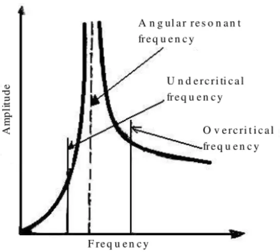
Establishing the most favorable vibration operation conditions for swinging screens is the essential problem when devising such equipment. The amplitude and the frequency of vibrations are the decisive factors that influence the vibrating conditions. The sieves operate best in over-critical angular resonant regime, at high frequencies coupled with small amplitudes for materials with a mainly fine grading, and at small frequencies coupled with high amplitudes for sorting materials with mainly coarse grading.

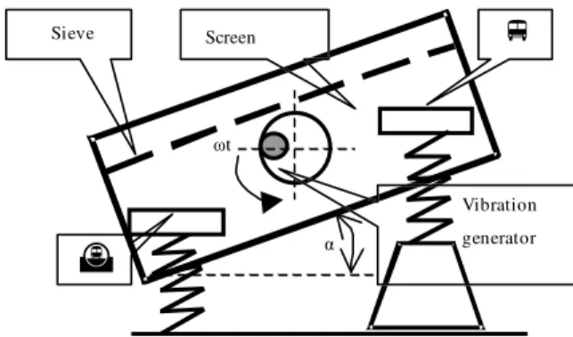
In the literature[1,2], there are guiding principles that recommend how to adopt the frequencies, the amplitudes, and how to adopt the dynamical conditions. The most used vibrating system in screening construction bulk material is the inertia one. In Fig. 1 the main components of such equipment are presented.

Screen

t Sieve

Vibration generator

F re q u e n c y

O v e r c ri t i c a l fr e q u e n c y U n d e r c r i ti c a l fr e q u e n c y A n g ul a r r e s o n a n t fr e q u e n c y

A

m

p

li

tu

d

e

Fig. 2: Over-critical vibratory regime

Fig. 3: The particle jump in the case when the jump is less than a complete sieve oscillation

an over-dose of bulk material occurs accidentally on the screen, the equipment presents a tendency to go to lower values of frequencies, and also, the amplitude to go to higher values Fig. 2. There is the advantage of obtaining an intense regime, and that will free faster the surface of the screen from the over-dose.

During a normal vibratory functioning regime, there are two periods of time from the point of view of the movements of the sieve: the first one (Interval index I in Fig. 3-4) in which the movement of the screen makes possible the acceleration, the deceleration and/or the stop of the particle movements on the screen surface, but the particle will stay all the time on this surface.

And a second one (Interval index II) in which the movement of the screen makes possible the jump of the particle from the surface of the screen.

Generally is accepted[1-3] that the sieve moves describe an ellipse. In this case, the equestion are Fig. 6,

Fig. 4: The particle jump in the case when the jump is as long as the complete sieve oscillation

(

)

( )

a sin t

b sin t

ξ = ⋅ ω + ε

η = ⋅ ω (1)

In formula (1), ξ-represents the elongation of the sieve motion on Oξ axis, η-represents the elongation of the sieve motion on Oη axis, a-represents the half of the amplitude of the movement on ξ-line, b-represents the half of the amplitude of the movement on η-line; ω -represents the angular frequency of the movement; ε- the difference of phase.

The acceleration in this case on η-line is:

( )

b sin t

η = − ⋅ ω ⋅ ω (2)

The maximum value of expression (2) is:

2 b

η = − ⋅ ω (3)

The expression of gravitation acceleration component on η-line is:

gη= ⋅g cosα (4)

In order to be able to define the movement conditions for each of those intervals, the throwing

coefficient (symbol c) can be used. The throwing

coefficient is defined as the minimum value of the ratio between the force capable to throw up the particle, and the gravity of this particle:

2 2

0

b sin t b 1

c

g cos g cos K

⋅ ω ⋅ ω ⋅ ω

= = =

⋅ α ⋅ α (5)

or several complete oscillations of the screen. This state of the jump is established[1,3] by the values of the throwing coefficient: for instance, the particle will begin to move only when the throwing coefficient c is greater that 1. That is because in sorting bulk material only a dynamical regime where the particle jumps over the surface is possible to adopt. That will give the first condition:

c>1 (6)

Also, this jump occurs[3] and takes place in the same time when the screen makes a complete oscillation. That will give the second condition:

2

c= 1+ π =3.29 (7)

There are also other conditions that must be realized, that imposed for the throwing coefficient other values, in order to obtain the best dynamical behavior for the screen. Other conditions to impose are:

• The particle in its jump must move higher than the thickness of the wire from which the sieve is made

• The length of the particle jump must be big enough the particle to pass at least in the next eye of the sieve,

• The dynamical regime must be sufficient to avoid a weak jump of the particle

So, from all these considerations the throwing coefficient must have, for the construction bulk materials, values in-between:

2.5≤ ≤c 3.25 (8)

We have two possible situations from the point of view of the particle’s movements on the sieve:

• The particle jump is less than a complete sieve oscillation, so the particle will move together with the sieve before another jump will occurs (Fig. 3)

• The particle jump is as long as the one complete sieve oscillation is. This is the ideal case, and means that the particle stays on the sieve only in the moment of its fall on the sieve, and immediately after the particle is thrown again by the sieve oscillation (Fig. 4)

The first regime is an ideal one. It might be present sometimes, but even if this regime is the one that is wanted and calculated, due to numerous variable factors

O₁

ξ η

Z

S

F_ηsin ωt

m_1g

m₂

m₁

O

k_ηk_ξ

F_ξsin (_ωt+_ε)

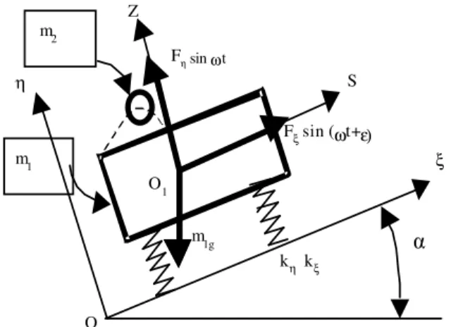
Fig. 5: Mobile axis (Z, S) and static axis (η, ξ) for the sieve-particle system

(such as the thickness of the material layer on the sieve, and the collisions in-between the particles inside the material layer, the moist of the material, etc.) after an ideal, long jump, several others short ones follow. The second regime is present almost permanently on the particle evolution on the sieve. So, it is preferable to adopt from the very beginning the first regime (Fig. 3), which is closer to the real phenomenon.

In order to build a mathematical model we consider such a mobile particle-screen complex as in Fig. 5, moving in the dynamic regime as in Fig. 3. In Fig. 5: the ηOξ axes are the motionless ones, and the zO1s axes

are the ones that move together with the sieve, m1

represents-the total mass of the screen, m2-the mass of

the particle, kη, kξ - the springs’ rates on Oη,

respectively, on Oξ axes. Also, generally the inertia screens have a gradient to assure a better fluidity of the material on the sieve.

In the Interval I (the particle and the sieve stay in contact), in the case of the movement of one single particle on the sieve of an inertia screen, as in Fig. 5, the screen movements are described by the next differential equation[2,3]:

1 2 1 2

k F

sin t g cos

m m m m

η η

η + ⋅ η = ⋅ ω − ⋅ α

+ + (9)

In Eq. (9), new dimensionless variables are introduced, variables defined in (10). In (10): z-represents dimensionless elongation, ω-represents the angular frequency of the movement of the screen, ω1

-represents the angular resonant frequency of the movement of the screen, k1-frequency coefficient, km

2

1 1

1 1

1 2 1

1 m 1

1

k m

z ; t ; ;

F m

m m g cos

k ; k ; n

m F

η

η

η

⋅ ω

= ⋅ η τ = ω ω =

ω ⋅ ⋅ α

= = =

ω

(10)

The dimensionless form of the Eq. (9) is defined in (11).

2 2 2 1 1 1 1 m m k k

z z sin k n

1 k 1 k

′′ + ⋅ = ⋅ τ − ⋅

+ + (11)

The Eq. (11) has the following solution:

(

)

z A sin

1 k

k B cos

1 k

k

sin n 1 k

1 k k

= ⋅ ⋅ τ +

+

⋅ ⋅ τ −

+

− ⋅ τ − ⋅ +

+ −

(12)

In the above Eq. (12), AI and BI represent the

integrating constants. The Eq. (12) represents the movement of the screen with the particle on the sieve in Interval I.

In Interval II, we have the equation of the movement of the sieve, without the presence of the particle on it:

1 1

k F

sin t g cos

m m

η η

η + ⋅ η = ⋅ ω − ⋅ α (13)

With the same new variables from (10), the Eq. (13) becomes:

2 2 2

1 1 1 1

z′′ +k ⋅ =z k ⋅sinτ −k ⋅n (14) This equation has the following solution (15):

(

)

(

)

II II 1 II 1

2 1

1 2

1

z A sin k B cos k

k

sin n 1 k

= ⋅ ⋅ τ + ⋅ ⋅ τ −

− ⋅ τ −

−

(15)

The Eq. (15) represents the movement of the screen without the particle on the sieve in Interval II. AII and

BII represent the integrating constants.

Similar considerations[3] lead us to the equation of particle movement during the jump over the sieve (16).

(

)

(

)

(

)

(

)

(

)

(

)

(

)

(

)

(

)

(

)

(

)

(

)

S II 1 0 1 0

II 1 0 1 0

2 1

0 0

2 1

II 1 1 0

II 1 1 0

2 1 0 2 1 2 2

1 1 0

S0 0

z A k cos k

B k sin k

k

cos 1 k

A sin k sin k

B cos k cos k

k sin sin 1 k k n z 2

= ⋅ ⋅ τ − τ ⋅ ⋅ τ −

− ⋅ ⋅ τ − τ ⋅ ⋅ τ −

− ⋅ τ − τ ⋅ τ −

−

− ⋅ ⋅ τ − ⋅ τ −

− ⋅ ⋅ τ − ⋅ τ +

+ ⋅ τ − τ −

−

⋅ ⋅ τ − τ

′

− + ⋅ τ − τ

(16)

The Eq. (16) represents the jump of the particle on the screen in Interval II. In this equation τ0 represents

the moment when the jump-starts and z’ SO represents

the speed of the particle in this moment.

In order to find the values of the constants AI, BI,

AII, BII, from the Eq. 12, 15 and 16 the initial states

are[3]:

• The continuity of the space: When the particle start the jump from the sieve surface (τ0), that is the

screen coordinates before (12), and immediately after the jump (15) are the same:

( )

( )

I 0 II 0

z τ =z τ (17)

• The continuity of the space: When the particle falls on the sieve surface (τc), after the jump, that is the

screen position before (15), and immediately after the falls (12), are the same:

( )

( )

II C I C

z τ =z τ (18)

• The continuity of the screen speed at the moment (τ0):

( )

( )

I 0 II 0

z′ τ =z′ τ (19)

• The expression of the sieve speed after the particle falls (a perfect plastic shock between the sieve surface and the particle is considered):

(

)

( )

( )

I C II C S C

m k

z 2 z z

1 k

′ τ − π = ′ τ + ⋅ τ

+ (20)

Fig. 6: The AIvalues (from [3] – pg 175, Fig.7.14)

Fig. 7: The BIvalues (from[3] pp: 175, Fig. 7.15)

( )

I 0 1 1

z′′ τ = −k ⋅n (21)

• The displacement of the particle in the moment of the fall on the sieve is null:

( )

S C

z τ =0 (22)

The initial states 17-22 will lead us to a system of 6 differential equations with 6 unknown parameters AI,

BI, AII, BII, τ0, τc.

All the involved equations are in transcendent form and it is necessary to solve the system by computer algorithms. Solving each times this system of equations is intricate, of course. There are some graphs[3] in order to find the necessary values for AI, BI, AII, BII,

(Fig. 6-9).

There is an important difficulty to assure the integration of all those factors in a one comprehensive mathematical model.

The main object of the present case of study is to adapt the existing system of Eq. 17-22 in order to be

Fig. 8: The AIIvalues (from[3] pp: 175, Fig. 7.17)

Fig. 9: The BIIvalues (from[3] pp: 175, Fig. 7.18)

able to build a numerical model to establish a best inertia vibratory regime in the case of sorting construction bulk materials. Starting from the above-mentioned system, a new system is made using linear expressions depending on throwing coefficient to replace the system integrating constants. The two systems are solved using the so-called false-position method for some usual sorting cases, and using the same initial conditions. Finally the results in those two cases are compared.

MATERIALS AND METHODS

It is obviously that the work with the diagrams to find values of interest of AI, BI, AII, BII, is not very

precisely, and also, working with the six equations system is not realistic in a day-to-day design work.

So, in order to make it easier to work with all these equations, the actual values of the integrating constants (corresponding to the construction bulk material) AI, BI,

AII, BII, obtained from the graphs in Fig. 6-9 was

Table 1: The values of integrating constants considered for linear interpolations

c AI BI AII BII

2.50 0.042 -0.400 -0.050 -0.168

2.55 0.050 -0.425 -0.040 -0.173

2.60 0.060 -0.440 -0.035 -0.175

2.65 0.080 -0.450 -0.032 -0.185

2.70 0.090 -0.465 -0.025 -0.190

2.75 0.110 -0.475 0.000 -0.195

2.80 0.120 -0.490 0.030 -0.200

2.85 0.140 -0.500 0.040 -0.205

2.90 0.143 -0.515 0.042 -0.210

2.95 0.147 -0.525 0.048 -0.215

3.00 0.150 -0.545 0.050 -0.220

3.05 0.154 -0.555 0.053 -0.215

3.10 0.156 -0.558 0.055 -0.215

3.15 0.159 -0.575 0.058 -0.210

3.20 0.160 -0.585 0.059 -0.210

3.25 0.162 -0.610 0.060 -0.210

3.30 0.165 -0.620 0.068 -0.215

parameters in Fig. 6-9 considered for linear interpolation are[4]: the throwing coefficient 2.5≤c≤3.3, the frequency coefficientk1 = 0.1, the mass coefficient

km = 0. In Table 1 are the AI, BI, AII, BII, values

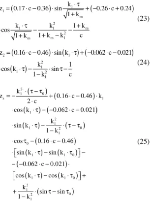
obtained. The linear interpolations were built with the corresponding built-in functions of MatLab program. The interpolations are illustrated in Fig. 10-13 (in the highlight windows are the interpolation equations). The new forms of Eq. are 23, 24 and 25.

(

)

(

)

1

m

2

1 1 m

2

m 1

m

k

z 0.17 c 0.36 sin 0.26 c 0.24

1 k

k k 1 k

cos

1 k k c

1 k

⋅ τ

= ⋅ − ⋅ + − ⋅ +

+

⋅ τ +

⋅ − − + − + (23)

(

)

(

) (

)

(

)

z 0.16 c 0.46 sin k 0.062 c 0.021

k 1

cos k sin

1 k c

= ⋅ − ⋅ ⋅ τ + − ⋅ −

⋅ ⋅ τ − ⋅ τ −

− (24)

(

)

(

)

(

) (

)

(

)

(

)

(

)

(

)

(

)

(

)

(

)

(

)

(

)

1 2 0

1

0

1 1 0

1 1 0

2 1 0 2 1 k

z 0.16 c 0.46 k

2 c

cos k 0.062 c 0.021

k sin k

1 k

cos 0.16 c 0.46

sin k sin k

0.062 c 0.021

cos k cos k

k

sin sin

1 k

⋅_{⋅ τ − τ}

= − + ⋅ − ⋅

⋅

⋅ ⋅ τ − − ⋅ −

⋅ ⋅ τ − ⋅ τ − τ

−

⋅ τ − ⋅ −

⋅ ⋅ τ − ⋅ τ −

− − ⋅ − ⋅

⋅ τ − ⋅ τ +

+ ⋅ τ − τ

−

(25)

The two systems of equations (first 12, 15, and 16, and second 23, 24, and 25) are both to characterize the movements of the particle-screen system at any moment.

2.5 2.6 2.7 2.8 2.9 3 3.1 3.2 -0.2 -0.1 0 0.1 0.2 Residuals

Linear: norm of residuals = 0.0538

2.5 2.6 2.7 2.8 2.9 3 3.1 3.2 3.3 0

0.05 0.1 0.15 0.2

Throwing coefficient "c"

V a lu e s o f A 1

A1 = f(c)

y = 0.17*x - 0.36

A1 linear

Fig. 10: The linear interpolation for AI

2.5 2.6 2.7 2.8 2.9 3 3.1 3.2 -0.1

-0.05 0 0.05

0.1 Residuals

Linear: norm of residuals = 0.017829

2.5 2.6 2.7 2.8 2.9 3 3.1 3.2 3.3 -0.7

-0.6 -0.5 -0.4 -0.3

Throwing coefficient "c"

V a lu e s o f B 1

B1 = f(c)

y = - 0.26*x + 0.24 B1 linear

Fig. 11: The linear interpolation for BI

2.5 2.6 2.7 2.8 2.9 3 3.1 3.2 -0.2 -0.1 0 0.1 0.2 Residuals

Linear: norm of residuals = 0.052597

2.5 2.6 2.7 2.8 2.9 3 3.1 3.2 3.3 -0.05

0 0.05 0.1 0.15

Throwing coefficient "c"

V a lu e s o f A 2 A2 =f(c)

y = 0.16*x - 0.46

A2 linear

Fig. 12: The linear interpolation for AII

2.5 2.6 2.7 2.8 2.9 3 3.1 3.2 -0.1 -0.05 0 0.05 0.1 Residuals

Linear: norm of residuals = 0.030574

2.5 2.6 2.7 2.8 2.9 3 3.1 3.2 3.3 -0.25

-0.2 -0.15

Throwing coeffcient "c"

V a lu e s o f B 2

B2 = f(c)

y = - 0.062*x - 0.021 B 2 linear

The two systems are in transcendent form and it is necessary to solve the system by computer algorithms. One of the available mathematical numerical possibilities is the so-called false-position method[4], valid because in both systems the functions are differentiable. A computer algorithm was made to find the values for the moments when the particles start the jump over the sieve (τ0), based on Eq. 17.

To apply the false-position method in this case, from (26) we build a new function, made by the difference between the two functions existing in (26).

(

)

(

)

(

)

1 1

I 0 I 0

m m

2 1

0 1 m

2

m 1

II 1 0 II 1 0

2 1

0 1

2 1

k k

A sin B cos

1 k 1 k

k

sin n 1 k

1 k k

A sin k B cos k

k

sin n

1 k

⋅ ⋅ τ + ⋅ ⋅ τ −

+ +

− ⋅ τ − ⋅ + =

+ −

= ⋅ ⋅ τ + ⋅ ⋅ τ −

− ⋅ τ −

−

(26)

The new function -g(τ0)-as show bellow, must be

null for the solution (in this case the throwing moment τ0):

(

)

(

)

(

)

1 1

0 I 0 I 0

m m

2 1

0 1 m II 1 0

2

m 1

2 1

II 1 0 2 0 1

1

k k

g( ) A sin B cos

1 k 1 k

k

sin n 1 k A sin k

1 k k

k

B cos k sin n 0

1 k

τ = ⋅ ⋅ τ + ⋅ ⋅ τ −

+ +

− ⋅ τ − ⋅ + − ⋅ ⋅ τ −

+ −

− ⋅ ⋅ τ + ⋅ τ + =

−

(27)

Now, a straight-line approximation to g (τ0) in the

range of two solutions [g (τ0 1), g (τ0 2)] is possible, and

we can estimate the root by linear interpolation (Fig. 14).

g(τ0)

g(τ0_1) g(τ0 s) g(τ0 2)

Fig. 14: The false-position method

After each iteration, a new domain is defined which incorporates the new found solutions so that [g (τ0 1), g (τ0 2)] always spans the root. That is, we replace

g (τ0 1) or g (τ0 2) by g (τ0 S), depending on its sign. The τ0_S formula is in Eq. (28) below:

(

)

0 _ S 0 _1 0 _ 2 0 _1

0 _ 2 0 _1

g( )

g( ) g( )

− τ

τ = τ + τ − τ ⋅

τ − τ (28)

RESULTS AND DISCUSSION

The values found for τ0, depending on the throwing

coefficient c, are shown in Table 2.

This calculus is made for the same screening conditions already mentioned: 2.5<c<3.3; k1 = 0.1,

km = 0.4.

The analysis that follows of the screen-particle system behaviour in the case of the two systems was done with values of the throwing coefficient that are important for construction bulk materials (that is 2.5≤c≤3.3). Using MatLab, the values of the functions zI,, zII, and zS from Eq. 12, 15 and 16 where overlapped

for each of the 17 values of the throwing coefficient in Table 2 (an example is illustrated in Fig. 15 for c = 2.5), and the same process was done for z1, z2, and zs

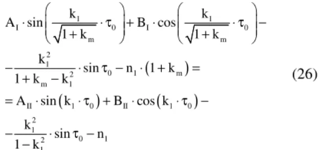
(Fig. 16). Another analysis was done also using MatLab, for the maximum values of the Eq. 12, 15, 16, 23, 24 and 25. The results in the case of Eq. 16 and 25 are illustrated bellow in Fig. 17 for 2.5<c<2.75, and in Fig. 18 for 2.8<c<3.3. Also, starting at the same jump moments, the particle falling locus was calculated in the two cases, using Eq. 16 and 25 (Fig. 19 are the results for the falling coordinates of the particles on the sieve for 2.5<c<2.75, and in Fig. 20 are the results for the falling coordinates for 2.8<c<3.3).

From the analysis of the overlapped graphs results that best trajectory are at values of the throwing coefficient in-between 2.5 and 2.75. For the values greater than 2.75 the trajectory of the particle is not high enough. One of the most important conditions for

Table 2: The values of 0

c 2.50 2.55 2.60

τ0 26.546 25.553 24.741

c 2.65 2.70 2.75

τ0 23.958 23.321 23.132

c 2.80 2.85 2.90

τ0 23.163 22.841 22.57

c 2.95 3.00 3.05

τ0 22.496 22.193 21.792

c 3.10 3.15 3.20

τ0 21.661 21.302 21.147

c 3.25 3.30

0 10 20 30 40 50 60 70 80 -3

-2.5 -2 -1.5 -1 -0.5 0 0.5

tau

Z

I

/

Z

I

I

/

Z

s

Particle jump - c = 2.5

Z I

jump moment z1(tauo)=z2(tauo) Z II

Zs

fall moment Zs(tauc)=0

Fig. 15:Overlapping of zI, zII and zS, for c = 2.5

(Eq. 12, 15 and 16)

0 10 20 30 40 50 60 70 80

-3.5 -3 -2.5 -2 -1.5 -1 -0.5 0 0.5

Particle jump - c = 2.5

tau

Z

I

/

Z

I

I

/

Z

s

Z I Z II Zs

Fig. 16: Overlapping of z1, z2 and zs, for c = 2.5

(Eq. 23-25)

-0.005 0 0.005 0.01 0.015 0.02 0.025 0.03

2.5 2.55 2.6 2.65 2.7 2.75

throwing coefficient

m

ax

im

u

m

v

al

u

es

o

f

th

e

ju

m

p

equation in A1,B1,A2,B2 equations in "c"

Fig. 17: Maximum values of zI from (12) and z1

from (23)

an optimal functioning regime is that the fall of the particle to be almost normal to the sieve surface. Without a high enough trajectory this request cannot be fulfilled.

0 0.005 0.01 0.015 0.02 0.025 0.03 0.035 0.04 0.045 0.05

2.8 2.9 3 3.1 3.2 3.3

t hrowing coefficient "c"

m

ax

im

u

m

v

al

u

es

o

f

th

e

ju

m

p

equat ions in A1,B1,A2,B2 equat ions in "c"

Fig. 18: Maximum values of zII from (15) and z2

from (24)

c=2 .7 c=2 .7 5

c=2 .5 c=2 .5 5 c=2 .6 c=2.6 5

c=2.5 c=2.5 5 c=2 .6

c=2 .7 5 c=2 .7

c=2 .6 5

-0 .8 4 -0 .8 3 -0 .8 2 -0 .8 1 -0 .8 -0 .7 9 -0 .7 8 -0 .7 7 -0 .7 6

6 0 61 6 2 6 3

t auc (falling m om ent s)

Z

I(

ta

u

c)

f

al

li

n

g

c

o

o

rd

in

at

es

equat io n in c equat io n s in A1 ,B1,A2 ,B2

Fig. 19: The falling coordinates of the particles on the sieve for the initial system (rhombus) and the new system (triangle) for 2.5≤c≤2.75

The maximum values of the particle jump are almost similar for both equations systems. Still, for values of the throwing coefficient in-between 2.8 and 3.3 there are some differences in the limits of around 10%.

c=2.8

c=3.2 c=3.3 c=3.25 c=3

c=3.05 c=3.15 c=3.1 c=2.85 c=2.9

c=2.95

c=3.3 c=3.25 c=3.2

c=3.15 c=3.1 c=3.05 c=3 c=2.95

c=2.9 c=2.85

c=2.8

-0.88 -0.86 -0.84 -0.82 -0.8 -0.78 -0.76 -0.74

58.8 59.8 60.8 61.8

tauc (falling m om ents)

Z

I

(t

au

c)

-f

al

li

n

g

c

o

o

rd

in

at

es

equations in A1,B1,A2,B2 equations in c

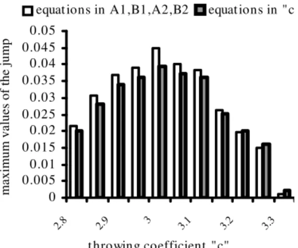
Fig. 20: The falling coordinates of the particles on the sieve for the initial system (rhombus) and the new system (square) 2.8≤c≤3.3

similar solutions, especially for the throwing coefficient values in-between 2.5 and 2.75. In the case 2.8 c 3.3 other values should be considered for k1 and km in order

to keep the sorting efficiency at high level. Generally, for construction bulk material the functioning frequency must be 10 times greater that the angular resonant frequency of the screen - this in highly necessary in order to avoid a slow crossing by resonant area, that can destroy the screen, sok1 should be around 0.1[4]. Also,

the mass of the material on the sieve should not be greater because the whole system became instable, that is a small over-dose of material can stop the vibrations or disturb the plane-parallel movements of the screen,

sokm should be around 0.4[4]. Finally it results that the

throwing coefficient used for equations in the case of construction bulk material must also be in the range of 2.5-2.75.

The new system is more convenient and easy to work with for devising sorting construction bulk materials processes. Another advantage is that in the very first steps one can choose the throwing coefficient and establish the best oscillations parameters.

REFERENCES

1. Mihailescu, St., 1983. Masini de Constructii si pentru Prelucrarea Agregatelor. Editura Didactica si Pedagogica, pag. 369-384. Machines in Civil Engineering and Aggregate Processing. Didactical and Pedagogical Publishing, pp: 369-384.

2. Munteanu, M., 1986. Introduction in the Dynamics of Vibrating Machines. Editura Academiei RSR, (RSR Academy Publishing, pp: 96-99).

3. Peicu, R.A., 1975. Studiul vibra iilor la ciururi în vederea stabilirii unor metode de calcul i proiectare, în scopul îmbun t irii coeficientului de calitate a cernerii. Tez de doctorat. Istitutul de Construc ii Bucure ti 1975. (Screens vibrations study with a view to establishing some calculus and design methods in order to optimized the sorting quality coefficient, PhD thesis, Civil Engineering University, Bucharest 1975).