Qualitative and Quantitative Features of Orbits of Massive Particles
and Photons Moving in Wyman Geometry
G. Oliveira-Neto∗
Departamento de Matem´atica e Computac¸˜ao, Faculdade de Tecnologia,
Universidade do Estado do Rio de Janeiro, Rodovia Presidente Dutra Km 298, P´olo Industrial,
CEP 27537-000, Resende, RJ, Brazil
G. F. Sousa†
Departamento de F´ısica, Instituto de Ciˆencias Exatas, Universidade Federal de Juiz de Fora, CEP 36036-330, Juiz de Fora, MG, Brazil
(Received on 20 July, 2008)
The Wyman’s solution depends on two parameters, the massMand the scalar chargeσ. If one fixesMto a positive value, sayM0, and letσ2take values along the real line it describes three different types of spacetimes. Forσ2>0 the spacetimes are naked singularities, forσ2=0 one has the Schwarzschild black hole of mass
M0and finally for−M02≤σ2<0 one has wormhole spacetimes. In the present work, we shall study quali-tative and quantiquali-tative features of orbits of massive particles and photons moving in the naked singularity and wormhole spacetimes of the Wyman solution. These orbits are the timelike geodesics for massive particles and null geodesics for photons. Combining the four geodesic equations with an additional equation derived from the line element, we obtain an effective potential for the massive particles and a different effective potential for the photons. We investigate all possible types of orbits, for massive particles and photons, by studying the appropriate effective potential. We notice that for certain naked singularities, there is an infinity potential wall that prevents both massive particles and photons ever to reach the naked singularity. We notice, also, that for certain wormholes, the potential is finite everywhere, which allows massive particles and photons moving from one wormhole asymptotically flat region to the other. We also compute the radial timelike and null geodesics for massive particles and photons, respectively, moving in the naked singularities and wormholes spacetimes.
Keywords: Wyman Geometry; Geodesics; Effective Potential; Naked Singularities and Wormholes
1. INTRODUCTION
Theweak equivalence principleof general relativity tell us that massive particles move along timelike geodesics and pho-tons move along null geodesics [1]. Despite their fundamental importance as one of the principles of general relativity, the geodesics also help us learning more about different proper-ties of a given spacetime. A textbook example comes from the study of geodesics in Schwarzschild geometry [1]. With-out actually computing the geodesics, just observing the effec-tive potential diagram, one can see that both massive particles and photons can never leave the event horizon once they enter that surface. This is the case because the effective potential for both massive particles and photons diverges to negative infinity as one approaches the singularity located at the ori-gin of the spherical coordinates. Therefore, once the massive particles and photons enter the event horizon they are accel-erated toward the singularity without any chance to turn back. Many authors, over the years, have computed the effective potential diagram and the geodesics of different spacetimes in order to learn more about their properties. In particular, we may mention some important works dealing with different
∗email:[email protected]
†email:gilberto [email protected]
black hole spacetimes [2]. Two other important gravitational configurations besides black holes that may form due to the gravitational collapse are naked singularities and wormholes. Some authors have already investigated some of their proper-ties by computing effective potential diagrams and geodesics for those spacetimes [3–5]. A well-known spacetime geome-try which may describe naked singularities as well as worm-holes is the Wyman one [6]. Since, to the best of our knowl-edge, nobody has ever computed effective potential diagrams and geodesics for the Wyman spacetime, we decided to do that in the present work.
studies of that model [15].
The Wyman’s solution is not usually thought to be of great importance for the issue of gravitational collapse because it is static and the naked singularities derived from it are unsta-ble against spherically symmetric linear perturbations of the system [9, 10]. On the other hand, as we saw above, from a particular case of the Wyman’s solution one may derive the Roberts’ one which is of great importance for the issue of gravitational collapse. Also, it was shown that there are nakedly singular solutions to the static, massive scalar field equations which are stable against spherically symmetric lin-ear perturbations [10]. Therefore, we think it is of great im-portance to gather as much information as we can about the Wyman’s solution for they may be helpful for a better under-stand of the scalar field collapse.
The Wyman’s solution depends on two parameters, the mass M and the scalar charge σ. If one fixesM to a posi-tive value, sayM0, and letσ2take values along the real line it describes three different types of spacetimes. Forσ2>0 the spacetimes are naked singularities, for σ2=0 one has the Schwarzschild black hole of mass M0 and finally for −M2
0 ≤σ2<0 one has wormhole spacetimes. Therefore, we have an interesting situation where we can study differ-ent properties of naked singularities and wormholes together through the effective potential diagrams and geodesics of mas-sive particles and photons in the Wyman’s solution.
In the next Section, we introduce the Wyman solution and identify the values of the parametersM andηthat describes naked singularities, wormholes and the Schwarzschild black hole. In Section 3, we combine the geodesic equations to ob-tain the effective potential equation for the case of massive particles. We study the effective potential and qualitatively describe the types of orbits for massive particles moving in the naked singularities and wormholes spacetimes. In this sec-tion, we also compute the radial timelike geodesics for parti-cles moving in the naked singularities and wormholes space-times. In Section 4, we combine the geodesic equations to obtain the effective potential equation for the case of photons. We study the effective potential and qualitatively describe the types of orbits for photons moving in the naked singularities and wormholes spacetimes. In this section, we also compute the radial timelike geodesics for photons moving in the naked singularities and wormholes spacetimes. Finally, in Section 5 we summarize the main points and results of our paper.
2. NAKED SINGULARITIES, WORMHOLES AND THE SCHWARZSCHILD BLACK HOLE.
The Wyman line element and the scalar field expression are given in coordinates (t,r,θ,φ) by equation (9) of [8],
ds2=−³1−2η r
´Mη
dt2+³1−2η r
´−Mη
dr2+
+³1−2η r
´1−Mη
r2dΩ2, (1)
wherervaries in the range 2η<r<∞anddΩ2is the line element on the unit sphere. The scalar field is,
ϕ= σ 2ηln
³ 1−2η
r ´
. (2)
whereσis the scalar charge given byσ2=η2
−M2andσ2 ≥ −M2. We are working in the unit system whereG=c=1.
In the line element (1), the functionR(r),
R(r) =r³1−2rη´
1 2(1−Mη)
, (3)
is the physical radius which gives the circumference and area of the two-spheres present in the Wyman geometry. Instead of using the parametersM andσto identify the different space-times described by (1), we may also use the parametersM andη, since they are all related by the equation just below (2). Each different spacetime will have a different behavior of R(r). R(r)has a single extremal value which is a minimum located atr=M+η. Since, the line element (1) is valid for r>2η, only whenM>ηthere will be a minimum inside the domain ofr. Based on that result we have three different cases for a positiveM. As a matter of simplicity we shall use, also, the positive parameterλ≡M/η.
Case M<ηor 0<λ<1.
In this case we have the following important values ofR(r) (3),
lim r→2η+
R(r) =0, lim
r→∞R(r) =∞. (4) Here, the solution represents spacetimes with a physical naked timelike singularity located atR=0 [7]. It is easy to see that this singularity is physical because, the Ricci scalarR
computed from the line element (1),
R=2(M
2 −η2) r4
³ 1−2η
r ´Mη−2
, (5)
diverges there. It is also easy to see that this singularity is naked with the aid of the quantityQ=gαβ ∂R∂xα∂x∂Rβ. The roots of
Qdetermine the presence of event horizons in spherical sym-metric spacetimes [12]. For the Wyman solutionQis given by,
Q=³1−2rη´−1³1−M+r η´2. (6) The only root ofQis located atr=M+ηwhich confirms that the singularity located atR=0 is naked for all spacetimes in the present case.
Case M=ηorλ=1.
In this case we haveR(r) =randσ=0. This last condi-tion implies that the scalar field (2) vanishes and one gets the Schwarzchild solution. Here, the minimum ofR(r), located at R=2M, is outside the domain ofrand the line element (1)
describes only the spacetime exterior to the event horizon.
Case M>ηor 1<λ<∞.
In this case we have the following important values ofR(r) (3),
lim r→2η+
R(r) =∞, Rmin= (M+η)
³M−η
M+η
´12(1−Mη) , lim
r→∞R(r) =∞. (7)
Due to the fact thatσ2≥ −M2as stated just before (2), we have that in the present caseη≥0. The case η=0 is well know in the literature as the Yilmaz-Rosen space-time [16]. In this case M>η, the physical radius R is never zero. If one starts with a large value ofR, for large values ofr, and starts diminishingR, reducing the values ofr, one reachs the minimum value ofR(Rmin(7)) forr=M+η. Then,Rstarts to increase again when we letr goes to 2ηuntil it diverges whenr=2η. Therefore, we may interpret these spacetimes as wormholes connecting two asymptotically flat regions such that they have a minimum throat radius given byRmin(7) [11]. The spatial infinity (R→∞) of each asymptotically flat region is obtained, respectively, by the limits: r→∞andr→2η+.
An important property of this space-time is that the scalar field (2) is imaginary. The imaginary scalar field also known as ghost Klein-Gordon field [17] is an example of the type of matter calledexoticby some authors [18]. It violates most of the energy conditions and is repulsive. This property helps explaining the reason why the collapsing scalar field never reachesR=0.
As mentioned above, in the rest of the paper we shall restrict our attention to the spacetimes representing naked singulari-ties and wormholes.
3. TIMELIKE GEODESICS
3.1. Effective Potential
We have four geodesic equations, one for each coordinate [1],
d2xα dτ2 +Γ
α βγ
dxβ dτ
dxγ
dτ =0, (8)
whereα=0,1,2,3, andxαrepresents, respectively, each of the coordinates (t,r,θ,φ).τis the proper time of the massive particle which trajectory is described by (8).
The geodesic equation for θ tell us that, like in the Schwarzschild case, the geodesics are independent ofθ, there-fore we choose the equatorial plane to describe the particle motion (θ=π/2). In the equatorial plane, the geodesic equa-tion forφcan be integrated to give,
r2³1−2η r
´1−Mη ˙
φ=R2φ˙ =L, (9) where the dot means derivative with respect toτandLis the integration constant that may be interpreted as the particle an-gular momentum per unit rest mass. This result means that φiscyclicand its conjugated momentum (pφ=φ˙) is a con-served quantity. Also, ˙φmay be written as a function ofr. Likewise, in the equatorial plane, the geodesic equation fort can be integrated to give,
³
1−2rη´
M η
˙
t =E, (10)
whereEis the integration constant that may be interpreted as the particle energy per unit rest mass. This result means thatt iscyclicand its conjugated momentum (pt=t˙) is a conserved quantity. Also, ˙tmay be written as a function ofr. Instead of using the fourth geodesic equation forr, we use the equation derived directly from the line element (1),ds2/dτ2=−1 [19]. There, we introduce the expressions of ˙φ(9) and ˙t (10), in order to obtain the following equation which depends only on r,
µdr
dτ
¶2
+V2(r) =E2. (11)
Where
V2(r) =³1−2η r
´Mη "
1+L
2
r2 ³
1−2η r
´Mη−1 #
(12)
andV(r)is the effective potential for the motion of massive particles in the Wyman geometry. The geodesic equation for rplays the role of a control equation, where we substitute the solutions to the other four equations, in order to verify their correctness.
first derivative ofV2(r)(12) and find the roots of the result-ing equation. That equation may be simplified by the intro-duction of the auxiliary quantities:x= (1−2η/r), 0<x<1; A=η2/L2, 0<A<∞;B= (λ−1/2)/(λ+1/2),−1<B<1; C=2λ/(λ+1/2), 0<C<2. Whereλwas defined before and the domains ofA,BandCwhere determined by the fact thatλis positive. The equationdV2(r)/dr=0, in terms ofx, λ,A,BandCis given by,
F(x)³ACx1−λ+B−Cx+x2´=0, (13) whereF(x) = [λxλ−1(1−x)]2/2ACM. Since F(x)6=0, for 0<x<1, the term between parenthesis will give the roots of eq. (13). Unfortunately, there are not algebraic expressions for all these roots. The use of numerical techniques, in the present case, would give the roots of eq. (13) only for precise numerical values of all the parameters present in that equa-tion. One would have to study each individual case, for each case is described by a different set of values of the parameters present in eq. (13). It is a possible way to solve eq. (13) but it would take a lot of computational time and effort. On the other hand, there is a mathematical treatment that allows the derivation of the algebraic expression of one root of eq. (13), in terms of λ. It, also, allows the identification of the exact number and nature (if it is a maximum, a minimum or a point of inflection ofV2(r)), besides the region in theλdomain, of all the other roots of eq. (13). Furthermore, that mathematical treatment reduces greatly the computational time and effort, mentioned above. It starts with the definition of the following two auxiliary functions,
p(x) = −x2+Cx−B, h(x) =ACx1−λ. (14) Now, the values ofxwhere the two curvesp(x)andh(x)meet will be the roots of (13). p(x)is a set of parabolas which ver-tices are all located above the x-axis and with two roots. The larger one is located atx=1 and the smaller one is located atx= (λ−1/2)/(λ+1/2). Forλ>1/2, the smaller root is positive; forλ=1/2, it is zero and forλ<1/2, it is nega-tive. The precise nature ofh(x)will depend on the value ofλ, present in the exponent ofx, but whateverλone chooses, all values ofh(x)will be located above the x-axis. Forλ>1,h(x) diverges to+∞whenx→0 and goes to zero whenx→+∞. Forλ<1,h(x)goes to zero whenx→0 and diverges to+∞ whenx→+∞.
An important root of (13) is defined by the value ofx, say x0, where the two curves p(x)andh(x)(14) just touch each other. x0is a point of inflection ofV2(r)(12), because there the second derivative ofV2(r)is also zero. Associated tox0 there is an angular momentum, sayL0, which originates an unstable particle orbit. Due to the fact thatLis present, only, in the denominator ofAin the expression ofh(x)(14), if one increasesL,h(x)will assume smaller values for the same val-ues ofx. p(x)will not be altered becauseLis not present in its expression. Therefore,L0is the value ofLfor whichh(x) just touchesp(x), if one takes values ofLgreater thanL0,h(x) will start intercepting p(x)in two or more points. They will
be extremal values ofV2(r): maximum, minimum or point of inflection. It is possible to compute the value ofL0in terms of x0 and the parameters λ andη. In order to do that, we consider, initially, the fact that the first derivatives ofh(x)and p(x)(14), inx=x0, are equal and expressACx0−λin terms of other quantities. Then, we use the fact thatx0is a root of (13) and rewrite that equation forx=x0 and substitute there the value ofACx−λ0 just obtained. It gives rise to the following second degree polynomial equation inx0,
x20− Cλ λ+1x0+
λ−1
λ+1B=0, (15) whereλ6=1. It has the following roots,
x+0 = 2λ
2+√5λ2−1
2(λ+1/2)(λ+1), x − 0 =
2λ2−√5λ2−1 2(λ+1/2)(λ+1),
(16) wherex+0 ≥x−0. Due to the fact that we have two distinct values ofx0,x+0 andx−0 given by (16), we shall have, also, two distinct values ofL0, sayL0+andL0−. In order to obtain them, we introducex0+andx−0, separately, in the equation that equates the first derivatives ofh(x)andp(x)and expressL20in term of other quantities. It gives,
L20+= η
2λ(1 −λ) (x+0)λ[λ−x+
0(λ+1/2)]
,
L20−= η
2λ(1−λ)
(x−0)λ[λ−x−
0(λ+1/2)]
, (17)
whereL20−≥L20+.
Sincex+0 andx−0 vary in the range[0,1]andL20+ andL20− must be positive, we will have to impose some restrictions on the domain ofλ. These restrictions lead to the following distinct domains ofλ, depending on which root one is using,
x−0 : √1
5 ≤λ< 1
2, (18)
x+0 : λ≥ √1
5. (19)
Therefore, this result tell us thatV2(r)(12) behaves differ-ently, depending on the value ofλ. We have the following three different regions:
(i)λ≥1/2.
There will be just one point of inflection located atx+0 for L20+. If one chooses values ofL2>L20+, one will find other extremal values ofV2(r)(12), which will be a maximum or a minimum.
(ii) 1/√5≤λ<1/2.
There may be two different points of inflection. The first is located atx+0 forL2=L2
L20+, one will find other extremal values ofV2(r)(12), which will be a maximum or a minimum. When one reachesL2=
L20−, one finds the other possible point of inflection located atx−0. If one chooses values ofL2>L20−, one will find just one extremal value ofV2(r)(12), which will be a minimum. Even for the caseL2<L2
0+, there will be a minimum. In fact,
this minimum will always be present for any value ofL. Its presence can be understood because, here,p(x)has a negative root and h(x)is crescent and starts from x=0. Therefore, these two curves will always intercept each other.
(iii)λ<1/√5.
There will be no point of inflection but there will be always a minimum. The presence of this minimum can be understood in the same way as the one in the previous case.
As we saw in the previous section, Sec. 2, naked singular-ities and wormholes are characterized by certain subdomains ofλ. Therefore, based on the above result, we may describe the effective potentials for naked singularities and wormholes.
3.2. Effective Potential for Naked Singularities
As we saw, in Sec. 2, the naked singularities are obtained for 0<λ<1. We may still divide the naked singularities in two classes, due to the behavior ofV2(r)(12) whenr→2η+.
Since the present naked singularity is a physical singularity, we expect thatV2(r)diverges there.
For 0<λ<1/2, limr→2η+V
2(r) =∞. Due to the fact that this limit is consistent with an asymptotically flat naked sin-gularity located atr=2η, we call this class of ordinary naked singularities.
On the other hand, for 1/2≤λ<1, limr→2η+V2(r) =0.
Due to fact that this result is not consistent with a naked sin-gularity located at r→2η, we call this class ofanomalous naked singularities. Then, in what follows we shall restrict our attention to the class of ordinary naked singularities with 0<λ<1/2. It is important to mention that observing the scalar field expression (2), which in this case is real, one can see that it diverges to−∞asr→2η+.
Taking in account the results of Subsec. 3.1 (ii) and (iii) the effective potentialV2(r)(12) may have several different shapes depending on the value ofL2. Here, the points of in-flection will be located at x−0 and x+0 (16) and the relevant angular momenta will beL20−andL20+(17).
• ForL2<L20+,V2(r)(12) has one minimum. In terms of xit is located in the range (0,x−0) or in terms ofrit is lo-cated in the range (2η,r−0 ≡2η/(1−x−0)). ForE2<1, the massive particles orbit around the naked singularity. If the massive particle is located exactly at the minimum the orbit is circular and stable. ForE2>1, the massive particles come in from infinity reach the infinity poten-tial wall near the naked singularity and return to infinity without ever reach the naked singularity.
• For L2=L20+,V2(r) (12) has two extremal values, a minimum located in the range (2η,r−0) and a point of inflection located atr=r+0 ≡2η/(1−x+0). In this point
the massive particles have unstable circular orbits. The other possible trajectories for the massive particles are exactly as in the previous case.
• ForL20+<L2<L20−,V2(r)(12) has three extremal val-ues, a minimum located in the range (2η,r0−), a maxi-mum located in the range (r0−,r+0) and another max-imum located in the range (r0+ , ∞). If the massive particles are exactly in the maxima they have unstable circular orbits. The other possible trajectories for the massive particles are exactly as in the first case.
• ForL2=L2
0−,V2(r)(12) has two extremal values, a minimum located in the range (r+0 ,∞) and a point of inflection located atr=r0−. In this point the massive particles have unstable circular orbits. The other possi-ble trajectories for the massive particles are exactly as in the first case.
• ForL2>L20−,V2(r)(12) has one minimum located in the range (r0+,∞). The possible trajectories for the mas-sive particles are exactly as in the first case.
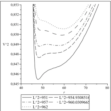
It is important to mention that, for sufficiently large values ofE, any massive particles will come in from infinity and it will get reflected by the infinity potential wall near the naked singularity. Then, it will return to infinity without ever reach the naked singularity. This result is similar to the one found in [4] for timelike geodesics of the naked singularity present in the Reissner-Nordstr¨om spacetime. Let us consider, as an example, the case whereM=10 andλ=0.45. Therefore, we haveL20+=954.9308516 andx+0 =0.1875874406 which in terms ofris given byr0+=54.70674220. We also have,L20−= 960.0309665 andx−0 =0.1064234487 which in terms ofris given byr−0 =49.73770224. In Fig. 1, we plotV2(r)(12) for each of the five cases discussed above. They have the five different values ofL2: 951, 954.9308516, 957, 960.0309665 and 962. The naked singularity is located atr=44.44444444.
3.3. Effective Potential for Wormholes
As we saw, in Sec. 2, the wormholes are obtained for 1<λ<∞. In the spatial infinity of each asymptotically flat region the effective potentialV2(r)(12) assumes the follow-ing values,
lim r→2η+
V2(r) =0, lim r→∞V
2(r) =1. (20)
Although the above limits give consistent values for the ef-fective potential at the two spatial infinities, the first limit is not consistent with the value of the Ricci scalar evaluated at r=2η, for wormholes with 1<λ≤2. For this class of worm-holes the Ricci scalarR(5), diverges to∞when we take the limitr→2η+or gives a positive constant whenλ=2. These
L^2=951 L^2=954.9308516 L^2=957 L^2=960.0309665 L^2=962
r
40 50 60 70 80
V^2
0,845 0,846 0,847 0,848 0,849 0,850 0,851 0,852 0,853
FIG. 1: Five different effective potential diagramsV2(r)(12), for massive particles moving in a naked singularity withM=10 andλ=
0.45. They have the five different values ofL2: 951, 954.9308516, 957, 960.0309665 and 962. The naked singularity is located atr=
44.44444444.
we call this class of wormholes ofanomalous wormholes. For the rest of the wormholes where 2<λ<∞, the limit of R
(5) whenr→2η+is zero. This value is consistent with the
first limit ofV2(r)in (20) and the idea of an asymptotically flat spatial region. Then, in what follows we shall restrict our attention to that class of ordinary wormholes with 2<λ<∞. Taking in account the results of Subsec. 3.1 (i) the effective potentialV2(r)(12) may have three different shapes depend-ing on the value ofL2. Here, the point of inflection will be located atx+0 (16) and the relevant angular momentum will be L20+(17).
• ForL2<L20+,V2(r)(12) has no extremal values. In this case, there is no stable orbits. For sufficiently high en-ergies the massive particles may travel from one asymp-totically flat region to the other. In fact, this type of orbit is also present in the next two cases.
• ForL2=L2
0+,V2(r)(12) has one point of inflection,
located atx+0 (16) or in terms ofr,r+0 ≡2η/(1−x+0). In this point the massive particles have unstable circular orbits.
• For L2>L20+,V2(r) (12) has two extremal values, a maximum located at 2η<r<r+0 and a minimum lo-cated at r+0 <r. There are closed and open orbits de-pending on the values of the total energy and angular momentum of the massive particles.
Let us consider, as an example, the case where M =1 and λ=√1000. Therefore, we have L2
0+=12.41266 and
L^2=10 L^2=12.41266 L^2=14.5 r
2 4 6 8 10 12 14 16 18 20
V^2
0,6 0,7 0,8 0,9
FIG. 2: Three different effective potential diagramsV2(r)(12), for massive particles moving in a wormhole withM=1 andλ=√1000. They have the three different values ofL2: 10, 12.41266 and 14.4. The spatial infinities of each asymptotically flat region are located at r=0.06325 andr→∞.
x+0 =0.98799 which in terms ofris given byr+0 =5.26747. In Fig. 2, we plotV2(r)(12) for each of the three cases dis-cussed above. They have the three different values ofL2: 10, 12.41266 and 14.4. The spatial infinities of each asymptoti-cally flat region are located atr=0.06325 andr→∞.
3.4. Radial timelike geodesics
Unfortunately, there is not an algebraic expression for the general timelike geodesics given by the solutions to Eqs. (9-11), even the numerical solutions are very complicated. On the other hand, one may restrict his attention to the case of radial timelike geodesics, where the massive particle moves only along the radial and time directions. It means that ˙θ= ˙
φ=L=0 and (11) reduces to,
µdr
dτ
¶2
=E2 −³1−2rη´
M η
. (21)
Although (21) is much simpler than (11), one still cannot obtain an algebraic expression ofτas a function ofr, after its integration. Therefore, we shall perform a numerical study of the solutions to (21) and present our results.
whenris large,rtends to a linear function of the proper time τ. ForE<1, the geodesics are also well behaved whenr→2η andτalso goes to zero in that limit. On the other hand, they do not extend to large values ofr. It is clear from (21), that the massive particles are subjected to a potential of the form:(1− 2η/r)M/η. This potential, increases from zero atr=2ηand tends to one whenr→∞. Therefore, massive particles with a total energyE<1, get reflected by the potential. The value of r, where the particle gets reflected by the potential is obtained by solving the equation: E2= (1−2η/r)M/η. Then, based on the above results, we may conclude that it always takes a finite proper time interval to travel from any finite value ofr to the singularity located atr=2η. We notice, also, that for radial timelike geodesics there is not an infinity potential wall near the naked singularity and the massive particles can reach it.
b. Wormholes In this case, we integrated (21) for many different values ofE,Mandη. We chose values ofMandη compatibles with wormholes. We found that, forE≥1, the geodesics are all well behaved whenr→2η. In fact,τgoes to zero in that limit. The geodesics are such that whenr is large, rtends to a linear function of the proper time τ. For E<1, the geodesics are also well behaved whenr→2ηand τalso goes to zero in that limit. On the other hand, they do not extend to large values ofrbecause they get reflected by the potential, as in the naked singularity case. The value ofr, where the particle gets reflected by the potential is obtained in the same way as in the naked singularity case. Here, as in the naked singularity case, for all cases studied it always takes a finite proper time interval to travel from any finite value ofr to the spatial infinity located atr=2η.
4. NULL GEODESICS
4.1. Effective Potential
The null geodesics for the Wyman solution are derived al-most in the same way the timelike geodesics were derived in the previous section. The only difference is that, here, the null line element contributes a different additional equa-tion to the four geodesic equaequa-tions. The new equaequa-tion reads: ds2/dχ2 =0, where χ is the affine parameter used in the present case. Therefore, proceeding exactly as in the previous section we obtain the following effective potential equation,
µdr
dχ
¶2
+V2(r) = 1
b2, (22)
where
V2(r) =r−2³1−2rη´
2M η −1
(23)
andb≡L/E is the photon impact parameter. V2(r)(23) is the effective potential for the motion of the photon in Wyman geometry.
V2(r)(23) has only one extremal value atr=2M+η. Due to the domain ofrit can only exists if 2M>ηor λ>1/2 and when it exists it is a maximum. Therefore, we have three different cases: (i)λ>1/2, the effective potential has a maxi-mum atr=2M+ηand goes to zero atr=2η;(ii)λ=1/2, the effective potential has no extremal values and diverges to∞as r→0; (iii)λ<1/2, the effective potential has no extremal values and diverges to∞asr→2η.
4.2. Effective Potential for Naked Singularities
As it was mentioned in Subsec. 3.2, we are only concerned, here, with the class of ordinary naked singularities character-ized 0<λ<1/2. For this class,V2(r)(12) assumes the fol-lowing values whenr→2η+andr→+∞,
lim r→2η+
V2(r) =∞, lim r→+∞V
2(r) =
0. (24)
V2(r)(23) has no extremal values. In this case, whatever the impact parameterbthe photons come in from infinity, get re-flected by the infinity potential wall near the naked singularity and return to infinity without ever reach the naked singularity.
4.3. Effective Potential for Wormholes
As it was mentioned in Subsec. 3.3, we are only concerned, here, with the class of ordinary wormholes characterized by 2<λ<∞. In the spatial infinity of each asymptotically flat regionV2(r)(23) assumes the following values,
lim r→2η+
V2(r) =0, lim r→∞V
2(r) =0. (25)
V2(r) (23) has a maximum located atr=2M+η. In this point the photons have unstable circular orbits. For suffi-ciently small impact parameterbthe photons may travel from one asymptotically flat region to the other. Otherwise, they come in from spatial infinity of an asymptotically flat region get reflected by the effective potential and return to spatial in-finity in the same asymptotically flat region.
4.4. Radial null geodesics
5. CONCLUSIONS.
In the present work, we studied qualitative and quantitative features of orbits of massive particles and photons moving in the naked singularity and wormhole spacetimes of the Wyman solution. We investigated all possible types of orbits, for mas-sive particles and photons, by studying the appropriate effec-tive potential. We noticed that for certain naked singularities, there is an infinity potential wall that prevents both massive particles and photons ever to reach the naked singularity. This result is similar to the one found in [4] for timelike geodesics of the naked singularity present in the Reissner-Nordstr¨om spacetime. We noticed, also, that for certain wormholes, the
potential is finite everywhere, which allows massive particles and photons moving from one wormhole asymptotically flat region to the other. We also computed the radial timelike and null geodesics for massive particles and photons, respectively, moving in the naked singularities and wormholes spacetimes. It is important to mention that, the above description of the radial timelike and null geodesics in terms ofτand χ may also be done in terms of the time coordinatet, leading to few different results [20].
Acknowledgments. G. Oliveira-Neto (Researcher of
CNPq, Brazil) thanks CNPq and FAPERJ for partial financial support and G F Sousa thanks CAPES for financial support.
[1] For a detailed explanation see: C. W. Misner, K. S. Thorne and J. A. Wheeler,Gravitation, (Freeman, New York, 1973). [2] M. J. Jaklitsch, C. Hellaby, and D. R. Matraversl, Gen. Rel.
Grav.21, 941 (1989); Z. Stuchl´ık and M. Calvani, Gen. Rel. Grav. 23, 507 (1991); Z. Stuchl´ık and S. Hled´ık, Phys. Rev. D60, 044006 (1999); J. Podolsk´y, Gen. Rel. Grav. 31, 1703 (1999); G. V. Kraniotis and S. B. Whitehouse, Class. Quant. Grav.20, 4817 (2003); G. V. Kraniotis, Class. Quant. Grav.21, 4743 (2004); N. Cruz, M. Olivares, and J. R. Villanueva, Class. Quant. Grav.22, 1167 (2005).
[3] J. M. Cohen and R. Gautreau, Phys. Rev. D19, 2273 (1979); Z. Stuchl´ık and S. Hled´ık, Class. Quant. Grav.17, 4541 (2000); Z. Stuchl´ık and P. Slan´y, Phys. Rev. D69, 064001 (2004). [4] A. Qadir and A. A. Siddiqui, Int. J. Mod. Phys. D16, 25 (2007). [5] J. C. Graves and D. R. Brill, Phys. Rev.120, 1507 (1960); M. Azreg-Ainou and G. Cl´ement, Gen. Rel. Grav.22, 1119 (1990). [6] M. Wyman, Phys. Rev. D24, 839 (1981).
[7] I. Z. Fisher, Zh. Eksp. Teor. Fiz.18, 636 (1948) and an English version available in gr-qc/9911008; O. Bergman and R. Leip-nik, Phys. Rev. D107, 1157 (1957); H. A. Buchdahl, ibid.111, 1417 (1959); A. I. Janis, E. T. Newman, and J. Wincour, Phys. Rev. Lett.20, 878 (1968); J. E. Chase, Commun. Math. Phys. 19, 276 (1970); A. G. Agnese and M. LaCamera, Lett. Nuovo Cimento35, 365 (1982); Phys. Rev. D31, 1280 (1985); D. D. Dionysion, Astro. Space Sci.83, 493 (1982); J. Froyland, Phys. Rev. D. 25, 1470 (1982); M. D. Roberts, Gen. Rel. Grav.17,
913 (1985); Class. Quant. Grav.2, L69 (1985); Astro. Space Sci.147, 321 (1988).
[8] M. D. Roberts, Gen. Rel. Grav.21, 907 (1989). [9] P. Jetzer and D. Scialom, Phys. Lett. A169, 12 (1992). [10] M. A. Clayton, L. Demopoulos, and J. Legare, Phys. Lett. A
248, 131 (1998).
[11] G. Oliveira-Neto and F. I. Takakura, J. Math. Phys.46, 062503 (2005).
[12] P. R. Brady, Class. Quant. Grav.11, 1255 (1994).
[13] Y. Oshiro, K. Nakamura, and A. Tomimatsu, Prog. Theor. Phys. 91, 1265 (1994).
[14] M. W. Choptuik, Phys. Rev. Lett.70, 9 (1993).
[15] D. Christodoulou, Commun. Math. Phys.105, 337 (1986);106, 587 (1986); 109, 591 and 613 (1987); Commun. Pure Appl. Math.XLIV339 (1991);XLVI, 1131 (1993); Ann. Math.140, 607 (1994).
[16] H. Yilmaz, Phys. Rev.111, 1417 (1958); N. Rosen, in Relativ-ity, eds. Carmeli, Fickler and Witten (New York, N. Y., 1970), 229.
[17] S. A. Hayward, S. W. Kim, and H. Lee, Phys. Rev. D65, 064003 (2002).
[18] M. S. Morris and K. S. Thorne, Am. J. Phys.56, 395 (1988). [19] R. A. D’Inverno, Introducing Einstein’s Relativity, (Oxford