Temporal Resources for Global Quantum Computing Architectures
Juan D. Jaramillo∗ and John H. Reina†
Departamento de F´ısica, Universidad del Valle, Apartado A´ereo 25360, Cali, Colombia
(Received on 3 April, 2008)
Using the methods for optimal simulation of quantum logic gates, we perform a quantitative estimation of the time resources involved in the execution of universal gate sets for the case of three representative models of quantum computation based on globalcontrol. The importance of such models stems from the solution to the problem of experimentally addressing and locally manipulating the qubits in a given quantum register. The numerical estimation of the temporal efficiency for each model is performed by assuming that the qubits in the register can be coupled to each other via the Ising and the F ¨orster interactions. Finally, we discuss the feasibility of the physical realization of such architectures under quantum error correction conditions.
Keywords: Quantum control; Quantum computation; Quantum error correction
1. INTRODUCTION
Quantum computation stands as one of the outstanding in-novations of current technologies. As Feynman pointed out almost five decades ago [1], the development of smaller elec-tronic devices ultimately leads to a consideration of quantum mechanical effects in electronic and computer designs [2]. Moreover, it became clear after the works of Deutsch [3] and Shor [4] that quantum mechanics could provide the means for a radical new way of computing, allowing the compu-tation of many intractable compucompu-tational problems in “clas-sical machines” (computers running under “clas“clas-sical” phe-nomenology), such as factoring of large numbers [4] or the exact simulation of large quantum systems [5]. Aside from the usual model of quantum circuits for quantum computation (QC) [3] there are other models under current investigation, such as one-way QC [6], adiabatic QC [7], quantum cellular automata [8], and others. Although these models are equiva-lent in the sense that they can simulate each other with polyno-mial slowdown in its time and space resources, when it comes to physical realizations, polynomial differences between mod-els become a relevant issue regarding error robusticity [9].
A problem of central importance is the necessity to charac-terize the efficiency of such models in different computational problems and for different physical systems. Qubit chains as-sociated with two level quantum systems interacting with their nearest neighbours are a common array for many QC mod-els. In these arrays, the input information is stored along with the subsequent evolution of the system. In order to perform any quantum computation on the register, it is sufficient to be able to realize a universal set of one and two-qubit quantum gates [10]. There are two main mechanisms for the implemen-tation of localized multi-qubit gates in a quantum register: the traditional ‘local’ control (LC) and the so-called ‘global’ con-trol (GC). In LC quantum computation (LCQC), an induced evolution in the system requires thedirectindividual localiza-tion of the computalocaliza-tional qubits. A problem common to such
∗Electronic address:[email protected]
†Electronic address:[email protected]
a strategy is the difficulty in its physical implementation, es-pecially at scales where the manipulation invokes more than a few qubits register. By contrast, in GC quantum computing (GCQC) the induced evolution of the system doesn’t require direct individual localization of the computational qubits to be targeted by the logic gates; the model manages to induce a localized gate by using the instructions stored in the register’s initial configuration. Thus, from the viewpoint of quantum in-formation technologies, it may be more promising to be able to realize unitary manipulations within the quantum register in a global fashion.
In this work, we evaluate the additional temporal resources required for the execution of three relevant architectures for GCQC [11–13]. Our results are based on a precise determi-nation of temporal resources by means of techniques based on time-optimal simulation of quantum gates [14, 15]. More-over, we also estimate the spatial resources involved in the conditional dynamics performance and discuss the feasibility of such architectures for implementing quantum error correc-tion over the computacorrec-tional and the auxiliary qubits consid-ered in Refs. [11–13].
2. TIME-OPTIMAL SIMULATION OF QUANTUM GATES
Calculation of optimal times for the execution of quan-tum gates depends specifically on the form of the interacting Hamiltonian between qubits. The optimal time execution of ann-qubits gate
U
, using a HamiltonianH
, is defined as theminimal timeTexecuting
U
in the controllable system [16]:˙
U(t) =−i
H
(t)U(t);U(0) =I;U(T) =U
, (1)whereU(t)belongs to the special unitary groupSU(2n),Iis the group’s identity element,T is the time it takes to go from Ito
U
alongSU(2n), andH
(t)≡H
0+H
Ctrl(t), (2)is a curve in the space of Hermitic matrices of dimensionn, decomposed as a sum of a time independent matrix
H
0 andis associated to a qubit-qubit interacting Hamiltonian (e.g., Eq. (6)) and the controllable term
H
Ctrl(t) to a local (one qubit) Hamiltonian, which could be physically realized, e.g., through the coupling with a controllable external magnetic field. In this work, we apply the techniques introduced in Refs. [14, 15] for treating quantum computer systems to the case of globally controlled systems. A central consideration here is thefast control limit[14, 15], by which the execution time of local Hamiltonians is considered “arbitrarily fast”, an assumption based on the experimental consideration that the strength of the coupling between the qubit and the control-lable external field can be raised high enough as to consider negligible the time of one qubit rotations in comparison with the time induced by the qubit-qubit interactions.Formally, this means that if we letG=SU(2n), andK be the subgroup ofGassociated to local unitary operations [16], i.e., unitaries with the form exp(−i
H
Ctrl), then1. The execution time for
U
is equivalent to that forKU
and
U
K.U
is said to belocally equivalentto ˜U
if thereexistk1, k2∈Ksuch that
U
=k1U
˜k2.2. Finding the optimal time for simulating a quantum gate
U
∈Gis equivalent to finding the geodesic betweenI andU
in the coset spaceG/K.Here, we focus on the results for two and three-qubit gates, which are the core of the considered GCQC protocols. Opti-mal time solutions for locally controlled systems of two-qubit gates have already been reported [14]. The conditions for an optimal simulation of a quantum gate
U
under an interactingHamiltonianH0can be reduced to finding the minimum time t[17], such that
~α≺S~βt, (3)
where~α and~β are coefficients characterizing the unitaries exp(−i∑ αiσi⊗σi) and exp(−i∑ βiσi⊗σi), which are
lo-cally equivalent to
U
and exp(−iH0)respectively, and theσi’sdenote the Pauli matrices. The special majorization relation ≺S is established in direct relation to the normal
majoriza-tion relamajoriza-tion between the vectors~λ and~ν associated to the eigenvalues of exp(−i∑ αiσi⊗σi) and exp(−i∑ βiσi⊗σi),
respectively. It is important to note that the previous ana-lytic solution relies on the fact thatSU(4)/(SU(2)×SU(2)) is a Riemannian symmetric space, which implies the exis-tence of an abelian subalgebra. This assures the charac-terization of locally equivalent operators based on unitaries of the generic form exp(−i∑ αiσi⊗σi). Regarding
three-qubit gates, optimal simulation results have only been found under specific situations [15, 18]. Here, the previous ap-proach is no longer valid: geodesics have to be solved in SU(8)/(SU(2)×SU(2)), which is not Riemannian symmet-ric. Important quantum gates such as theCNOT andSWAP between the first and the third qubit have been solved by a combination of analytical and numerical techniques [15, 18]. Other quantum gates, such as the ones we apply in this work, are indirectly addressed by decomposition into already solved quantum gates.
3. MODELS FOR QUANTUM COMPUTATION BASED ON
GLOBAL CONTROL
The GCQC models are arrays of two level quantum systems interacting, in first approximation, with their nearest neigh-bours. There exists a finite number of “qubit species” dis-tributed in an alternate manner within the arrays, as shown schematically in Fig. 1(a). Here, each species can be collec-tively manipulated in an independent way. An example of a physical realization of such architectures is a linear array of coupled quantum systems which has associated a periodic and finite set of frequencies (ωA,ωB,ωA,· · ·) that can be addressed
through resonant radiofrequency (RF) pulses. Between the ‘computational’ qubits, those effectively involved in the com-putation, there are auxiliary qubits or “ancillae”, with purely operative functions which are initialized in the computational state|0i⊗m. Besides the ancillae, there is a “special qubit”, the “control unit”, whose role it is to localize and ‘transport’ in-formation between the computational qubits. One qubit gates, for example, are performed in two steps: first, the control unit is taken near enough to the computational qubit to be modi-fied, and then the desired gate is performed over the compu-tational qubit, as a controlled gate, where the control unit acts as the control qubit.
We next introduce the three architectures and the respective operative protocols that we use in our calculations.
i) Model 1 (BM1). Proposed by Benjamin [11], this is one of the simplest models for GCQC; it consists of two species ofphysicalqubits,AandB, as shown in Fig. 1. The computational qubits are encoded in physical qubits (|0i ≡ |↑i and|1i ≡ |↓i) belonging exclusively to a given species with the exception of the “special qubit” or “control unit”, which is initialized in a different species at the computational state |1i. There are arrays of three and five ancillae qubits alternately distributed between the computational qubits (see Fig. 1(b)). The generic Hamiltonian for this system is given by H =∑nj=1Hsj+∑nj=1Hintj,j+1, where the first term is associated with the individual qubit energy and the latter with the interaction energy between neighbouring qubits. The particular characteristics of the system reduce the total Hamiltonian to the form [11]:
H2j = HA,
H2j+1 = HB, H2j,2j+1 = HAB,
H2j+1,2j = HBA. (4)
This model works as long as the following conditions are ful-filled: a) it has to be possible to control the supression of the interaction process due toHBA, in a way that the system
view [19]. To alleviate such difficulties, a strategy that incor-porates a third energy level as part of one of the qubit species (a “barrier”), has been put forward in Ref. [19], at the cost of increasing the number of species in the array.
‘
Ti
me
st
ep
Ctrl-U (A)B
(c) (a)
(b)
FIG. 1: (a) Schematic of a periodic array of two types of qubits (A
andB), present in the architecturesBM1andBM2(see text) for quan-tum computation based on global control. (b) Array of ancillae and computational qubits in architectureBM1. (c) One qubit gateU
act-ing selectively on qubitY. The gate is indirectly performed using the controlled quantum gateCtrlB(A), which uses theHABinteraction
Hamiltonian. The “control unit” acts as the control qubit and assures the localized action ofU. Adapted from Ref. [11].
As an illustration, in Fig. 1(c) we show how to perform a one computational qubit gate: the control unit is located at an adjacent cell from the target qubit (Y). Making sure that the interacting Hamiltonian between the target and the control unit is turned on (HAB), any arbitrary controlled gate
(Ctrl−
U
) can be performed by means of using the specieswhere the control unit is located as thecontrolqubit and the species where the target computational qubit is located as the target.
ii)Model 2(BM2). This model actually precedesBM1[12]. It has the same Hamiltonian configuration specified in Eq. (4). Unlike BM1, this model doesn’t require the ability to independently control the interacting Hamiltonians, HAB and HBA. This benefit doesn’t come free; in this case the
computational qubits are encoded in four physical qubits, as follows: |0i ≡ |↑↑↓↓iand|1i ≡ |↓↓↑↑i. Between every en-coded computational qubit there are four ancillae qubits. The “control unit” is also encoded, but in a different configuration: |↑↑↓↓↑↑iand|↑↑↑↑↑↑i, representing the computational states |1i and |0i, respectively. The complete array is shown in Fig. 2(a). The operational gates which, applied sequentially, perform any computational gate, are symmetric three qubit gates of the generic form
M(u00,u01,u10,u11) = |00i h00| ⊗u00+|01i h01| ⊗u01+ |10i h10| ⊗u10+|11i h11| ⊗u11,
(5)
whereM acts simultaneously over every physical qubit of a given species and the symmetric conditionu01=u10 is ful-filled. This condition is compatible with the fact that neigh-bouring qubits are of the same species and therefore only sym-metric gates are physically feasible.
Z Y W V
Z Y W
V CU
CU
Y Y
a
b
c
(a) Entanglement
(b) ctrl-U (V)
(c) Undo Entanglement Y
Ti
m
e
Y Y
(a)
(b)
FIG. 2: (a) Array of ancillae and computational qubits in architecture
BM2. (b) Heuristic protocol for two-qubit (VandY) computational gates in modelsBM1andBM2. Computational qubits are in light gray and distinguished by letters. The white space between compu-tational qubits corresponds to ancillae qubits, and the line in dark grey corresponds to the control unit path. Adapted from Ref. [12].
Here, there’s no need to control interacting Hamiltonians and computational qubits are encoded in physical qubits belonging exclusively to a given species, just as in BM1. There are two ancillae qubits between the computational qubits.
A B C B C A B C A B C
W 0 1 X 0 0 Y 0 0 Z 0 0
0 W 1 X 0 0 Y 0 0 Z 0 0
0 W X 1 0 Y 0 0 Z 0 0 0
0 X W 1 Y 0 0 Z 0 0 0 0
0 0 0 X 0 0 Y W 1 Z 0 0
...
...
...
...
A
(1) (2) (3) (4)
(5)
Ti
me
st
ep
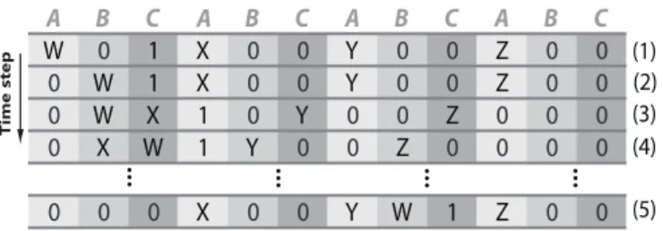
FIG. 3: Protocol for a two-qubit quantum gate between arbitrary computational qubitsW andZ, in architecture LM3. Every com-putational qubit is initiated at qubit speciesA. (1) The control unit is located at the neighbourhood ofW, in this caseWis at speciesA, while the control unit is at speciesC. (2) A controlledSWAPgate between speciesAandBis applied by using qubits at speciesCas the control qubits. Given the location of the control unit, only the computational qubitWwill be transferred to speciesB. (3) ASWAP
gate is applied between speciesAandC. (4) ASWAPgate is applied between speciesBandC. (5) Steps 2, 3, and 4 are applied again. The register is ready to implement a two-qubit gate between com-putational qubitsWandZusing the control unit. This is done after applying a controlled two-qubit gate between speciesAandB, where the speciesCacts as the control qubit. Any other operation can be reverted so that the modified computational qubitsWandZcan go to their initial locations in the register.
The operative gates that add up to perform computational gates are non-symmetric three qubit gates of the generic form given by Eq. (5). Unlike the models above, two-qubit gates are performed by the transportation of one of the computational qubits to a position adjacent to the second computational qubit involved in the two-qubit gate. This process, illustrated in Fig. 4, is performed by using the control unit to exclusively transport the first computational qubit (W) through the regis-ter. Once the control unit and the two computational qubits (WandZ) are all in the same neighbourhood,ABC, the sys-tem is ready to apply any two-qubit computational gate, where only the former computational qubits are involved. This is as-sured given that the control unit acts as a control qubit for the action of the two-qubit gate over the former computational qubits.
4. RESULTS AND DISCUSSION
For the evaluation of the growth of parameters regarding the number of computational qubits, the number of ancillae qubits between the computational qubits and the number of physical qubits required to codify a computational qubit were taken into account. The evaluation of the time performance of computational gates in the three architectures is based on the results of optimal simulation of quantum gates discussed in Section 2 [14, 15]. In a general picture, we consider quan-tum registers under global control, for which an anisotropic
Heisenberg interaction mediates the process of non-local gat-ing:
H
int =∑
iJXY(σix⊗σix+1+σiy⊗σyi+1) +JZσiz⊗σiz+1, (6)
which contains both the planarXYor F¨orster interaction (JZ=
0), and the isotropic Heisenberg interaction (JZ=JXY) as
lim-its.
4.1. Space and time scaling factors
We first consider a register for which there is an effective Ising interaction
H
int ≡H
Isingbetween neighbouring qubits:JZ≡J,JXY =0. Spatial scaling analysis is concerned with
the relation between the number of computational qubits,N, and the number of physical qubits, Np. The three models
scale linearly with respect to the total number of computa-tional qubits, and the proporcomputa-tionality factor,k, betweenNpand
Nis the unique parameter characterizing the spatial scaling in the three architecures.
Model LM3 3N Model BM2 8N Model BM1 4N
TABLE I: Average spatial scaling for the three architectures as func-tion of the number,N, of computational qubits.
Spatial scaling factors, without taking into account quan-tum error correction nor parallel processing, are given in Ta-ble I. The modelLM3 presents the best spatial efficiency with a scaling factork=3, followed byBM1, with the aver-age scaling factork=4. The modelBM2presents the worse comparative efficiency,k=8, due to the fact that besides the ancillae qubits, every computational qubit is encoded in four physical qubits.
architecture CH∗
Ising(
U) time (µs)
LM3 [441.6(n+m) +92.0]J−1 10.7
BM2 (403.2n+134.4m+1065.6)J−1 24.0
BM1 (28.2n+9.4m+15.6)J−1 0.25
TABLE II: Additional cost for the realization of one (n=0, neglect-ing all constant terms) and two computational qubit gates for the three models as a function of the Ising coupling strengthJ. The last column reports the associated time forJ=50 MHz.
Table II shows the results of the calculation of the time per-formance of general two-qubit computational gates i.e., gates where both computational qubits may be affected, for each architecture implemented under the Ising
H
Ising interactionHamiltonian. In this table,CH∗ Ising(
U
)represents the optimaladditional time spent in the execution of the arbitrary two-qubit gate
U
under the couplingH
Ising, and using GCQCmeaning, but for LCQC arrays. This initial choice of an Ising type of interaction is motivated by the following: i) given the heterostructural nature of the GCQC models, a non-resonant interaction is expected to be the most efficient interaction; ii) results for optimal simulation of three qubit quantum gates has only been developed for Ising type of interactions [15, 18].
There are two time scale factors in Table II: g1 andg2, which are associated to the two transportation processes rep-resented bynandmrespectively. The variablemis associated with the localization of one of the qubits involved in the com-putational gate by the control unit, andnto the transportation of the information between the two computational qubits in-volved in the gate execution. The model BM1 exhibits the best time efficiency with factorsg1=28.2 andg2=9.4. The fact that, forBM2andBM1, general two-qubit computational gates have to be realized by the action of two controlled gates, triples the magnitude of the factorg1.
The additional timesCH∗ Ising(
U
)are shown in Table II. Forthe purpose of illustration, specific times were calculated for the case m=0 and n=1 (control unit and computational qubits adjacent to each other) under coupling strength J= 50 MHz≈33 neV, which is a common order of magnitude for magnetic dipolar interactions in proposals such as fullerene-based electron spin quantum computers [20, 21]. The results are shown in Table II. For the three models, the one with lesser additional time spent isBM1, with a specific value of 0.25µs. Just for the sake of comparison, this is equivalent to 5.3 times the optimal time required in the direct realization of theSWAP gate, which performs the exchange of quantum states between qubits [22], and which, forJ=50 MHz, is 47.1 ns, as re-ported in Table IV. In contrast, the greater additional time, due to BM2, presents an extra cost equivalent to 509 times the direct application of theSWAPgate. In the case ofBM2 andBM1the same rates are found in comparison with the di-rect execution of theCNOTgate, given thatCH∗
Ising(SWAP) =
3CH∗
Ising(CNOT)andCHIsing(SWAP) =3CHIsing(CNOT). The
first equation comes from the observation that for BM1and BM2the additional computational time of general two-qubit gates, where both qubits are affected, triple that of a two-qubit controlled gate. The latter equation is directly deduced from Table IV.
modelBM1 time (ps) (14.1n+4.7m+15.6)JF−1 13.3
TABLE III: Additional cost for the realization of one (n=0,m=1) and two computational qubit gates in the modelBM1for the F¨orster coupling strengthJF. The second column gives the required time for
JF=1.5 THz.
Next, we compute the optimal additional time for general computational two-qubit gates for the case of a generic phys-ical system where the qubits interact via the F¨orster coupling: JXY ≡JF,J=0 in Eq. (6) [23–26]. We do so for the model
BM1. The calculation for the modelsLM3andBM2remains an open question due to the fact that optimal simulation for three qubit quantum gates under F¨orster interaction is still, hitherto, an unsolved problem. TheJF coupling appears in
many different physical systems, ranging from nanostructures such as quantum dots and wells [23–26] through to biomolec-ular systems [27–29]. The first column of Table III shows the general result associated to an arbitrary coupling intensityJF.
The last column shows the result forJF=1.5 THz≈1 meV,
which is a representative estimate for exchange interactions between quantum dots [23–26]. In this case, the parameters of “transport”g1andg2decrease by a factor of one half, ex-pressing the fact that the F¨orster interaction is a more efficient interaction for energy transfer.
U CH
Ising(
U) time (ns)
SWAP (3π/4)J−1 47.1
CNOT (π/4)J−1 15.7
U CH
F(
U) time (fs)
SWAP (3π/8)JF−1 775
CNOT (π/4)JF−1 516
TABLE IV: General and specific temporal costs for the direct execu-tion of theSWAPandCNOTquantum gates under the i) Ising and ii) F¨orster interaction Hamiltonians. The last column is computed for couplings i)J=50 MHz (33 neV) and ii)JF =1.5 THz (1 meV),
respectively.
To illustrate this point, in Table IV we show the optimal time for the execution of the two-qubit logic gatesSWAPand CNOT. TheSWAPgate is involved in the transportation of the computational qubits along the quantum register inBM1. The CNOTgate applies the quantumNOTgate (quantum version of the classicalNOT gate) conditioned by the computational state of its neighbouring qubit. We see from Table IV that CHF(SWAP)is one half timesCHIsing(SWAP)forJ=JF. The
factor 15.6 of Table III , which is independent of the processes of transportation, remains the same as that of Table II be-cause this only contains controlled gates which have the same generic value for both, Ising and F¨orster, couplings (see Ta-ble IV).
The additional time spent in the execution of a general two-qubit gate between neighbouring computational two-qubits un-der the F¨orster couplingJF=1.5 THz is approximately 17.2
times the optimal time required for the execution of theSWAP gate and 8.6 times the one required in the direct execution of theCNOT gate, under the same coupling conditions (see Table IV). The difference of five orders of magnitude in the optimal time required for the direct two-qubit gate execution between systems interacting under Ising and F¨orster coupling relies on the difference in their corresponding coupling in-tensities as taken from some representative systems such as fullerene-based electron spin quantum computers [20, 21] and systems of quantum dots coupled via exchange interactions [23, 26].
section is dedicated to a discussion of the implementation of quantum error correction in the three GCQC models presented above.
4.2. Quantum Error Correction
The overall additional resources required for these archi-tectures have important effects on their ability to implement quantum error correction codes (QECCs) [31]. In fact, fault-tolerant thresholds impose minimal values for coupling inten-sities between adjacent qubits. Calculation of these thresh-olds depends on the specific architecture and error correction strategies to be used [32], and some key observations can be made in this respect. Quantum error correction in GCQC models can be divided into two subproblems: i) quantum error correction of computational qubits and ii) classical error cor-rection of ancillae qubits. The problem of quantum corcor-rection of computational qubits may be solved by QECCs [22] but the implementation of QECCs in GCQC models is not a straight-forward process. For example, contrary to what is suggested in Ref. [33], computational qubits in the modelBM2cannot be corrected by QECCs because their architectural encoding doesn’t match with any QECC. To illustrate this, let us try to correct one computational qubit from abit-fliperror using the stabilizers formalism [22].
(a)
|q1i Z |p1i
|q2i Z Z |p2i
|q3i Z |p3i
|0i H • H |d1i
|0i H • H |d2i
(b)
input diagnostic output
{|000i,|111i} |00i {|000i,|111i} {|001i,|110i} |01i {|000i,|111i} {|100i,|011i} |10i {|000i,|111i} {|010i,|101i} |11i {|000i,|111i}
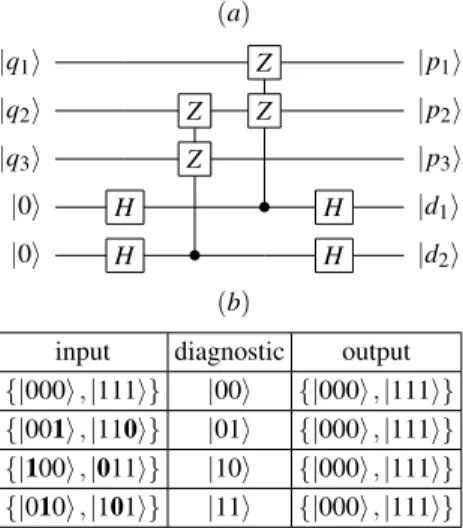
FIG. 4: (a) Error diagnostic code for thebit-flipone qubit error. (b) Input, diagnostic, and output for the QECC.
Figure 4 shows the diagnostic circuit using the set {Z2Z3,Z1Z2}as the stabilizer generators. One computational qubit is encoded into three physicalqubits in the following form: |0ic≡ |000iand|1ic≡ |111i. This circuit detects and therefore corrects all one bit-flip errors. Figure 4(b) shows the set (input) of correctable encoded qubits. However, in or-der to implement the bit-flip QECC inBM2, one has to encode each qubit,|qii, into four physical qubits following the
alloca-tion given by the architecture:|0i ≡ |↑↑↓↓i, and|1i ≡ |↓↓↑↑i. This leads to a total of twelve physical qubits per computa-tional qubit encoded. It is easy to check that any one
phys-icalqubit bit-flip error over an encoded computational qubit doesn’t belong to the set of correctable encoded qubits de-picted in Fig. 4(b). The same argument is valid to show the inability ofBM2to correct computational qubits through any other QECC. In fact, the only cases where QECC is possible in QC models witharchitecturalencoded qubits is when this encoding matches that of the QECC.
For the other models analyzed here, QECC is possible as long as a degree of parallelism of at least
O
(log(N))isfeasi-ble [34]. This fact makes the design of complementary strate-gies allowing parallel QECC processing inLM3 andBM1 a must. A strategy has already been put forward forBM1[32], using periodically distributed “switching stations” where con-trol units are activated and deactivated, except one, which is always activated and is used for the computation of the ac-tual algorithm. Parallel processing onLM3 hasn’t yet been explored.
The second issue, that of ancillae qubit correction, is an in-volved problem. As the aim of error correction on ancillae is to keep the ancillae qubits in their ground state,|0i, correc-tion is in this case to be carried out by dissipative operacorrec-tions over the register, also known as “resetting”. To achieve this, it has recently been proposed to consider a third level for each qubit, such that it could be populated from either of the states |0i and|1i, and would decay in a dissipative way into one particular state, say|0i[12, 32]. Aside from this, one more question remains: how to distinguish ancillae from computa-tional qubits? In the case ofLM3, computational qubits are naturally distinguished by the species they are, in a given time step. InBM1, this is not the case, because there are always ancillae qubits in the same species where the computational qubits are. A second alternative is to use the control unit to localize ancillae corrections, an effective strategy but less efficient compared to the one forLM3, where parallelism is maximal. Thus, parallel processing is necessary for QECC implementation inLM3andBM1, and the physical require-ment of a third energy level for each qubit will certainly be a common requirement inBM1andLM3in order to allow par-allel QECCs, if strategies such as those proposed in Refs. [12, 32] are to be implemented.
5. CONCLUSIONS
6. ACKNOWLEDGEMENTS
We are grateful to COLCIENCIAS for financial support un-der research contracts 1106-14-17903 and 1106-45-221296,
and the scientific exchange program PROCOL (DAAD-Colciencias).
[1] R. P. Feynman, “There is plenty of room at the bottom”, talk given by Richard Feynman on December 29, 1959, at the meet-ing of the American Physical Society at Caltech.
[2] R. P. Feynman, Int. J. Theor. Phys.21, 467 (1982).
[3] D. Deutsch, Proc. R. Soc. Lond. A400, 97 (1985); ibid.425, 73 (1989).
[4] P. W. Shor, Proceedings of the 35th symposium on Foundations of Computer Science, IEEEComputer Society Press, pp. 124 (1994).
[5] C. Zalka, Proc. R. Soc. Lond. A454, 313 (1998).
[6] R. Raussendorf and H. J. Briegel, Phys. Rev. Lett.86, 5188 (2000).
[7] E. Farhi, J. Goldstone, S. Gutmann, J. Lapan, and A. Lundgren, Science292, 472 (2001).
[8] C. A. Perez-Delgado and D. Chueng, e-print arxiv: quant-ph/0508164.
[9] A. M. Steane, Nature399, 124 (1999).
[10] D. P. DiVincenzo. Phys. Rev. A51, 1015 (1995). [11] S. C. Benjamin, Phys. Rev. Lett.88, 017904 (2002). [12] S. C. Benjamin, Phys. Rev. A61, 020301 (2000). [13] S. Lloyd, Science261, 1569 (1993).
[14] G. Vidal, K. Hammerer, and J. I. Cirac, Phys. Rev. Lett.88, 237902 (2002).
[15] N. Khaneja, R. Brockett, and S. J. Glaser, Phys. Rev. A 65, 032301 (2002).
[16] N. Khaneja, R. Brockett, and S. J. Glaser, Phys. Rev. A 63, 032308 (2001).
[17] K. Hammerer, G. Vidal, and J. I. Cirac, Rev. A 66, 062321 (2002).
[18] N. Khaneja, B. Heitmann, A. Spoerl, H. Yuan, T. Schulte-Herbrueggen, and S. J. Glaser, e-print arXiv: quant-ph/0605071.
[19] S. C. Benjamin, B. Lovett, and J. H. Reina, Phys. Rev. A70,
060305(R) (2004).
[20] W. Harneit, Phys. Rev. A65, 032322 (2002).
[21] S. C. Benjamin, A. Ardavan, A. Briggs, D. A. Britz, D. Gun-lycke, J. Jefferson, M. Jones, D. F. Leigh, B. W. Lovett, A. N. Khlobystov, S. A. Lyon, J. Morton, K. Porfyrakis, M. R. Sambrook and A. M. Tyryshkin, J. Phys.: Condensed Matter18, 867 (2006).
[22] M. A. Nielsen and I. L. Chuang, Quantum Information and Computation, Cambridge University Press (2000).
[23] J. H. Reina, L. Quiroga, and N. F. Johnson, Phys. Rev. A62, 012305 (2000).
[24] B. W. Lovett, J. H. Reina, A. Nazir, B. Kothari, and A. Briggs, Phys. Lett. A315, 136 (2003).
[25] B. W. Lovett, J. H. Reina, A. Nazir, and A. Briggs, Phys. Rev. B68, 205319 (2003).
[26] A. Nazir, B. Lovett, S. Barrett, J. H. Reina and A. Briggs, Phys. Rev. B71, 045334 (2005).
[27] T. Renger, V. May, and O. K¨uhn, Phys. Rep.343, 137 (2001). [28] G. S. Engel, T. R. Calhoun, E. L. Read, T.-K. Ahn, T. Mancal,
Y.-C. Cheng, R. E. Blankenship, and G. R. Fleming, Nature 446, 782 (2007).
[29] H. Lee, Y.-C. Cheng, and G. R. Fleming, Science316, 1462 (2007).
[30] J. H. Reina, L. Quiroga and N. F. Johnson, Phys. Rev. A65, 032326 (2002).
[31] A. M. Steane, Phys. Rev. Lett.77, 793 (1996). [32] A. Kay, e-print Arxiv: quant-ph/0702239.
[33] A. Bririd, S. C. Benjamin, and A. Kay, e-print Arxiv: quant-ph/0308113.