Solution of the Atmospheric Diffusion Equation with Longitudinal Wind
Speed Depending on Source Distance
Davidson Martins Moreira
1, Taciana Toledo de Almeida Albuquerque
2 1Centro Integrado de Manufatura e Tecnologia, Serviço Nacional de Aprendizagem Industrial,
Salvador, BA, Brazil.
2
Universidade Federal de Minas Gerais, Belo Horizonte, MG, Brazil.
Received: 20/3/2015 - Accepted: 23/7/2015
Abstract
An integral semi-analytical solution of the atmospheric diffusion equation considering wind speed as a function of both downwind distance from a pollution source and vertical height is presented. The model accounts for transformation and removal mechanisms via both chemical reaction and dry deposition processes. A hypothetical dispersion of contami-nants emitted from an urban pollution source in the presence of mesoscale winds in an unstable atmospheric boundary layer is showed. The results demonstrate that the mesoscale winds generated by urban heat islands advect contaminants upward, which increases the intensity of air pollution in urban areas.
Keywords:urban heat island, mesoscale wind, semi-analytical model, atmospheric boundary layer.
Solução da Equação de Difusão Atmosférica com Vento Longitudinal
Dependente da Distância da Fonte
Resumo
Neste trabalho, é apresentada uma solução integral semi-analítica da equação de difusão atmosférica considerando a velocidade do vento como função da distância longitudinal e vertical da fonte poluidora. O modelo leva em consideração os mecanismos de remoção e transformação via deposição seca e reação química. Uma hipotética fonte de emissão de contaminantes urbana na presença de ventos de mesoescala em uma camada limite instável é mostrada. Os resultados sugerem que os ventos de mesoescala gerados pela ilha de calor urbana advectam os contaminantes para cima, aumentando a intensidade da poluição atmosférica em áreas urbanas.
Palavras-chave:ilha de calor urbana, vento de mesoescala, modelo analítico, camada limite atmosférica.
1. Introduction
The atmospheric dispersion equation has long been used to describe the transport of air contaminants in a turbu-lent atmosphere. Analytical and semi-analytical solutions to this equation were the first and remain the most conve-nient methods for modeling air pollution because many at-mospheric problems can be studied. However, little atten-tion has been given to the atmospheric problems to find solution of this equation for wind speed as a function of both downwind distance (x) from the source and the
verti-cal height (z) above the ground, mainly due to the
mathe-matical complexity problem involved. We are aware of an-alytical and semi-anan-alytical solutions existence in the
literature, but for specific and particular problems. Among them, we mention the works of Rounds (1955), Smith (1957), Scriven and Fisher (1975), Demuth (1978), van Ulden (1978), Nieuwstadt and de Haan (1981), Sharanet al. (1996), Lin and Hildemann (1997), Wortmann et al.
(2005), Sharan and Modani (2006), Sharan and Kumar (2009). In all of these models, the wind speed is either a power law or logarithmic profile of vertical height and, similarly, the eddy diffusivity has been assumed either a power law or a parabolic profile ofzor a function of down-wind distance from the source. However, none of these pro-vides a systematic approach to find the solution with the generalized functional forms of wind speed and eddy diffu-sivity. At this point, it is important to mention that a
solu-Artigo
tion of the advection-diffusion equation can be written an integral form and also in series formulations with the same main property that both solutions are equivalent (Moreiraet al., 2010). Furthermore, analytical and semi-analytical
so-lutions are very important to understand and describe the physical phenomenon, since they are able to take into ac-count all the parameters of a problem and investigate their influence. Besides, while the preexisting numerical models require improvements for addressing more realistic situa-tions, it is helpful to first examine a few possible analytical (or semi-analytical) solutions to obtain a framework and a set of test solutions. These solutions are useful for a variety of applications, such as providing approximate analyses of alternative pollution scenarios, conducting sensitivity anal-yses for investigating the effects of various parameters or processes involved in contaminant transport, extrapolation over large time scales and distances where numerical solu-tions may be impractical, serving as screening models or benchmark solutions for more complex transport processes that cannot be solved exactly, and for validating more com-prehensive numerical solutions to the governing transport equations.
Focusing our attention in this direction, the novelty of this work consists of a semi-analytical solution of a two-dimensional advection-diffusion equation considering lon-gitudinal wind speed depending on thexandzvariables in
an air pollution problem. The literature does not present ex-perimental data to compare with the solution obtained in this work. Thus, to compare with a solution obtained in this work we use the results obtained by Agarwal and Tandon (2010), that present a numerical solution to the two-dimensional advection-diffusion equation considering an idealized situation with wind speed depending onxandz
variables. This idealized study tries to show the effect of ur-ban heat islands on urur-ban air pollution through mathemati-cal modeling. An attempt at such a solution is presented here in the form of a steady state two-dimensional mathe-matical model that allows for examining the dispersion of air contaminants in the urban atmosphere under the cumu-lative effect of large-scale and mesoscale winds. The two-dimensional heat island problem is an idealization; the mesoscale winds considered in the present study are only representative of a special type of wind.
The remainder of this paper is organized as follows. In section 2, the solution of the advection-diffusion equa-tion is presented. In secequa-tion 3, numerical results are re-ported. Lastly, in section 4, the conclusions of this study are presented.
2. The Model
It is well known that an analytical or semi-analytical solution can be expressed in either an integral or series for-mulation (Moreiraet al., 2010). Assuming that these
solu-tions are equivalent, results attained from an integral solution that considers the longitudinal wind speeds as a
function of x and z variables and realistic vertical eddy
diffusivity are presented in air pollution problems. For a Cartesian coordinate system in which thex
di-rection coincides with the didi-rection of the mean wind, the steady state advection-diffusion equation can be written as follows (Moreira and Vilhena, 2009):
u c
x v
c
y w
c
z x K
c x y K c y x y ¶ ¶ ¶ ¶ ¶ ¶ ¶ ¶ ¶ ¶ ¶ ¶ ¶ 
+ + = æ
è ç ö ø ÷ + æ è
çç öø÷÷+ æèç ö
ø ÷ -¶ ¶ ¶ ¶ l z K c z c z (1)
wherecdenotes the averaged concentration,u,v, andware
the mean wind speeds in thex(longitudinal),y(lateral) and z(vertical) directions,Kx,KyandKz(in this study
depend-ing only onz) are the eddy diffusivities in the respective
di-rections andlis a constant first-order depletion parameter that considers the relevant removal mechanisms, such as chemical reactions, rainout/washout, and artificial mecha-nisms that prevail in the atmosphere. To obtain the semi-analytical solution proposed in this study, Eq. (1) is inte-grated from -¥to +¥(c®0fory®-¥andy®+¥) in the
cross-wind direction (neglecting longitudinal diffusion, be-cause the advection transport term in thexdirection is
dom-inant over the diffusive term) to obtain the following relationship (Moreira and Vilhena, 2009):
u c
x w z z K
c z c y y z y y ¶ ¶ ¶ ¶ ¶ ¶ ¶ ¶ l
+ = æ
è
çç öø
÷÷-c
(2)
wherecyis the integrated cross-wind concentration.
In this study, the contaminant is transported horizon-tally by a large-scale wind, which is assumed to be function of altitude, and also function of the horizontal and vertical mesoscale winds. The mesoscale winds represent local winds that are caused by a heat source, which is an infinite cross-wind linear heat source parallel to the contaminant source in this study. For details see the works of Dilley and Yen (1971) and Agarwal and Tandon (2010). Therefore, the Eq. (2) can be written as follows:
(u u ) c
x w
c
z z K
c z c l e y e y z y y
+ + = æ
è
çç öø
÷÷-¶ ¶ ¶ ¶ ¶ ¶ 
¶ l (3)
whereulis the large-scale wind in thex(horizontal)
direc-tion andueandweare the mesoscale wind components in
thexandzdirections, respectively.
The heat island effect of a city causes air to rise above the center of the heat island. This rising air produces a sur-face influx of air from the surrounding area; large thermally induced convective currents are also generated (Dilley and Yen, 1971). These effects produce mesoscale winds.
In this work, the large-scale windulis parameterized
as a function of heightzin the manner suggested by Lin and
u u z u z z
l r
r
= = æ
è çç öø÷÷
( )
a
(4)
whereuris the measured wind speed at a reference heightzr
andais a constant that depends on the atmospheric stabil-ity. The mathematical formulations of the mesoscale hori-zontal and vertical wind components within the range of valid values are used as suggested by Dilley and Yen (1971). Thus, the following relationships are used in this study:
u ax z
z
e
r
= - æ
è çç öø÷÷
a
(5)
and
w az z
z e r = + æ è çç öø÷÷
(a )
a
1 (6)
whereais a proportionality constant (unit: 1/s). The expres-sions forul,ueandweare utilized within the surface layer.
Above this layer, these values are considered to be constant with height.
Furthermore, the wind speed component represented in Eq. (3) can be written as follows:
u u u z
z ax
z z
ax u
l e r
r r
r
+ = æ
è
çç öø÷÷ - æèçç öø÷÷ =
-æ è çç öø÷÷
a a
1 z
zr u u x z
r
æ è
çç öø÷÷ =
a
( , )
(7)
andu(x, z) = f(x).g(z), where f x axu
r ( )= -æ
è
ç ö
ø ÷
1 is a
non-dimensional function andg z u z z zr
( )= ( )= æ è
ç ö
ø ÷
a
is a
di-mensional function [LT-1].
The vertical eddy diffusivityKzis parameterized as a
function of heightzfollowing the work of Moreiraet al.
(2005b):
K K z w h z
h
z h
z h
z = z =
æ è
ç ö
ø
÷ æ
-è ç ö ø ÷ ´ - æ è ç ( ) . exp * 022 1 1 4
1 3 1 3
ö ø
÷ - æ
è ç ö ø ÷ é ë
ê 00003. exp 8hz ùûú
(8)
whereh is the atmospheric boundary layer (ABL) height
and w* is the convective velocity. The eddy diffusivity
parameterization is based on turbulent kinetic energy spec-tra and Taylor’s diffusion theory.
To solve Eq. (3), both source and boundary condi-tions are needed. Therefore, zero flux is assumed at the ground and at the top of the ABL. Moreover, a source with
emission rateQat heightHsis also assumed to obtain the
following:
K c
z z h
z y
׶ = =
¶ 0 at (9.a)
K c
z V c z z
z y
d y
׶ = =
¶ at 0 (9.b)
and
(ul u ce) ( , )z Q z H( ) x
y
s
+ 0 = d - at =0 (10)
wherez0is the roughness length,Vdis the deposition
veloc-ity anddis the Dirac delta function.
By considering the dependence of theKz(z) and wind
speed (i.e.,u(x,z) andw(z)) profiles on heightz, the height
of the ABLh is discretized intoNsub-intervals such that
within each interval, the average values in the vertical are used. Therefore, the solution to Eq. (3) is reduced to the so-lution ofNequations of the following type:
u c x w c z K c z c
z z z n N
n n y e n n y n n y n y n n ¶ ¶ ¶ ¶ ¶ ¶ l + = -£ -£ + = 2 2
1, 1:
(11)
wherecn
ydenotes the concentration,
we
nis the average
verti-cal mesosverti-cale wind and Kn is the average vertical eddy diffusivity, in thenthsub-interval. Moreover,
u f x
z z g z dz f x u
n n n n z z n n = - = + +
ò
( ) 1 ( ) ( )
1
1
(12)
and
f x ax
ur j x
( )= -æ ( )
è
çç1 öø÷÷ = (13)
A change of variables is used to obtain a solution to Eq. (11) (Crank, 1979, Moreiraet al., 2014). The new space
variablex*is defined by the following transformation:
x dx j x u a ax u r r x *
( ) ln
= ¢
¢ = -
-æ è çç öø÷÷
ò
10
(14)
The dimension ofx*is same asx[L]; therefore,x*is
considered to be a new space variable. Becausej(x) > 0, the
functionx®x*is an increasing function ofxthat vanishes atx= 0. Thus, the nature of the condition atx= 0 does not change in the new domain.
However, before providing additional details regard-ing the solution procedure, the obtained solution to Eq. (11) is valid only for the downwind range 0 <x<ur/aof the
large-scale and mesoscale winds; however, the range of va-lidity increases as the mesoscale winds approach zero.
u c x w c z K c z c n n y e n n y n n y n y ¶ ¶ ¶ ¶ ¶ ¶ l * + = -2 2 (15)
To account for vertically inhomogeneous turbulence (dependent onz), continuity conditions are imposed for the
concentration and concentration flux at the interfaces:
cn c n N
y n
y
= +1 =1 2, , , (K -1) (16.a)
and
K c
z K
c
z n N
n n y n n y ¶ ¶ ¶ ¶ = + + = -1
1 1 2, , , ( 1)
K (16.b)
These conditions must be considered to uniquely de-termine the 2Narbitrary constants appearing in the solution
to the set of equations defined in Eq. (15).
Applying the Laplace transform to Eq. (15) results in the following relationship:
d
dz c s z
w K
d
dzc s z
u s
K c s z
n e n n n n n n 2 2 ) ) ) ( , ) ( , ) ( ) ( , ) - -+ = -l u
K c z
n
n n
y( , )0
(17)
where)
c s zn L cp n x z x s
y
( , )= { ( *, ); *® }, which has the well-known solution (for details see work of Moreira et al.
(2006)):
)
c s z A e B e
Q
R e e
n n
R z n
R z
n
R z H R z H
n n
n
s n s
( , ) ( ( ) ( = + + -- -1 2 1 2 3
)) (18)
where R w K w K u s K n e n n e n n n n 1
2 1 2
1 2
1 2
4
= + æ
è
çç öø÷÷ + +
é ë ê ê ù û ú ú
( l)
R w K w K u s K n e n n e n n n n 1
2 1 2
1 2
1 2
4
= - æ
è
çç öø÷÷ + +
é ë ê ê ù û ú ú
( l)
and
Rn w K u s
e n
n n
3
2 4 1 2
=[( ) + ( +l)]
Finally, a linear system for the integration constants is generated by applying the interface and boundary condi-tions. Henceforth, the concentration is obtained by numeri-cally inverting the transformed concentration:
[
c x z
i e A e B e
Q R e n y sx n R z n R z i i n R n n ( , ) ( * * = + + - ¥ + ¥
ò
1 2 1 2 3 p g g1n z Hs R2n z Hs
s
e H z H ds
(- ) - (- )) ( - )ù û ú
(19)
whereH(z–Hs) is the Heaviside function. The integration
constantsAnandBnare previously determined by solving
the linear system resulting from the application of the boundary and interfaces conditions. Due to the complexity of the integrand, the line integral in Eq. (19) is evaluated numerically using the Fixed Talbot (FT) algorithm (Abate and Valkó, 2004). This procedure yields the following:
c x z r
M c r z e
e c s
n y n y rx x S n y k k ( , ) ( , )
Re ( ( )
* * ( ) * * = é ëê + 1 2 q q
[
, )( ( ))]
*z i k
k M 1 1 1 + ù û ú =
-å
t q(20)
where
s k r i
k k k k k
( ) (cot ),
( ) ( cot )cot
q q q + p q p
t q q q q q
= - < < +
= + -1
and
qk kp
M
= *
Moreover,x*is defined by Eq. (14),ris a parameter based on numerical experiments (r= 2M*/5x*) andM*is the number of terms in the summation.
The stepwise approximation of a continuous function converges to the continuous function when the individual steps in the approximation approach zero. For this study, it is necessary to choose an appropriate number of sub-layers by considering the smoothness of the functions forK,uand w. The solution obtained is semi-analytical in the sense that
the only approximations considered along its derivation are the stepwise approximation of the coefficients and the nu-merical Laplace inversion of the transformed concentra-tion. Therefore, this model preserves the beauty of a solution of the advection-diffusion equation without com-promising the accuracy of the wind speeds and the eddy diffusivity to compute the concentration.
3. Numerical Results
To illustrate the aptness of the formulation discussed for simulating contaminant dispersion in the ABL, the per-formance of the solution is evaluated hereafter. The present study primarily focuses on the concentration distribution of air contaminants in a given region under the influence of large-scale and mesoscale winds. The mesoscale winds are chosen to simulate local winds produced by urban heat is-land effects. The profiles of large-scale winds, mesoscale winds and the eddy diffusivity that are defined in Eqs. (4), (5), (6), (7) and (8) include several unknown parameters,
i.e.,ur,zr,a,a,w*andh. Therefore, these parameters are
re-quired as input to calculate the concentrations using the proposed scheme. The following values are assumed:
ur= 3 m/s;zr= 10 m, anda= 0,002 s-1. Moreover, the values
de-termined according to the stability conditions. In this work, only unstable atmospheric conditions are considered. Therefore, the following constants are assumed in the simu-lations performed:a= 0.17 (Agarwal and Tandon, 2010),
w*= 1 m/s andh= 500 m. The parameters above are chosen to represent a “light large-scale wind”. Thus, a compara-tively low value ofu= 3 m/s is used for the large-scale wind at 10 m. The value ofawas chosen to produce wind speeds in the region of interest that do not exceed the large-scale wind speeds. The contaminants are assumed to be emitted at a constant rate from a line source over an urban region. The simulated region extends from the origin and lies within the range of validity,i.e., 0 <x<ur/a(~1500 m).
It is assumed that the removal of contaminants occurs via ground absorption (dry deposition) and chemical reac-tions; these processes are defining the parametersVdandl,
respectively. For the purposes of this study,Vd= 0.6 cm/s
andlranges from 0 to 10-4s-1.
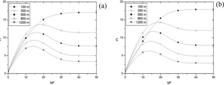
Figure 1 shows the numerical convergence of the pro-posed solution for the nondimensional ground-level con-centration (C = cyuh/Q, where u = urfor all simulations
performed) at various dimensional distances from the sour-ce (x= 100, 300, 500, 800 and 1200 m) for an increasing
number of terms in the summation (M*).
Figure (1a) shows convergence for simulations with-out mesoscale winds, while Fig. (1b) shows convergence for simulations with mesoscale winds. From these figures,
M*= 50 provides good accuracy for both cases. With the
in-crease of the number of terms in the numerical integration the solution stabilizes in a fixed value, that is, converges to one value, obeying certain numerical convergence criteria.
To obtain insight into the distribution of contaminants in a region that is simultaneously affected by both large-scale and mesolarge-scale winds under unstable atmospheric conditions, the computed concentrations are shown in Figs. (2-7). The analysis considers the contaminant
concen-tration distributions both with and without mesoscale winds to clearly visualize the effect of urban heat island on contaminant dispersion.
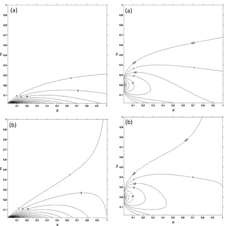
Figure 2 presents the isolines of the nondimensional concentrations (C = cyuh/Q) as a function of the
nondi-mensional distanceX(X=xw*/uh) and the nondimensional
heightZ (Z = z/h) for a ground-level source. Figure (2a)
shows the concentrations without mesoscale winds, while Fig. (2b) shows the concentrations with mesoscale winds.
An analysis of the results demonstrates the effects of the mesoscale winds on contaminant dispersion. For the case shown in Fig. (2b), the concentrations increase as the nondimensional source distance increases.
Figure 3 presents the isolines of the nondimensional concentrations as a function of the nondimensional dis-tance with a source atz/Hs= 0.2 (Hs= 100 m). Figure (3a)
shows the concentrations without mesoscale winds, while Fig. (3b) shows the concentrations with mesoscale winds.
Again, the effects of the mesoscale winds on contami-nant dispersion can be observed in the results. Figure (3b) shows that the concentrations increase as the nondimen-sional source distance increases.
Figure 4 shows the resulting vertical profile of the contaminant concentrations for a ground-level source at different distances from the source for the cases (a) without mesoscale winds and (b) with mesoscale winds.
According to Fig. 4, there is a greater tendency to-wards vertical homogenization in the contaminant concen-trations for the case with mesoscale winds.
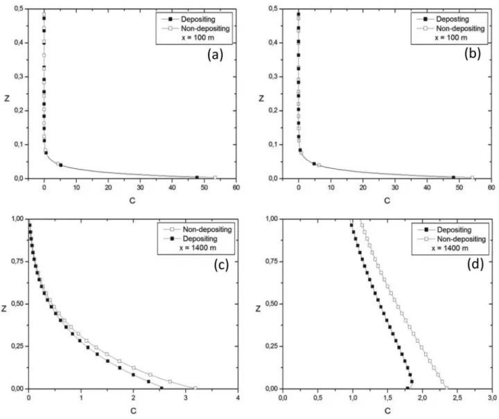
Figure 5 shows the effect of deposition for different distances (x= 100 m and 1400 m) and considering simula-tions with mesoscale winds and without mesoscale winds.
According to Fig. 5, for distances closer to the source (x= 100 m), dry deposition has less effect on the vertical profile concentrations for both scenarios. However, for greater distances from the source (x= 1400 m), the
ence on dry deposition is more evident in the vertical pro-file concentrations when considering the effect of meso-scale winds.
Figure 6 shows the effect of chemical reactions (l= 0, 10-3, 10-2, and 10-1) on the nondimensional concentrations vs.the nondimensional distance from the source at the
sur-face.
According to Fig. 6, the maximum concentration is greater in the case with mesoscale winds. Moreover, the concentrations decrease more rapidly as the distance from
the source increases despite the fact thatlis an order of magnitude smaller than in the case without mesoscale winds.
These figures are drawn with and without mesoscale winds; the results show that the concentration of air con-taminants is intensified due to the effects of mesoscale winds. These illustrations also show that the contaminant concentrations increase in the presence of mesoscale winds even at relatively high levels (especially compared with the case without mesoscale winds). The mesoscale winds cir-culate the contaminants and move the contaminants
up-Figura 3- Isolines of the nondimensional concentrations (C=cyuh/Q) as a function of the nondimensional distance (X =xw*/uh) and the
nondi-mensional height (Z=z/h) (source atz/Hs= 0.2) (a) without mesoscale
winds and (b) with mesoscale winds.
Figura 2- Isolines of the nondimensional concentrations (C=cyuh/Q) as a
function of the nondimensional distance (X=xw*/uh) and the
Figura 4- Vertical profile of the concentrations (C=cyuh/Q,Z=z/h) for dimensional distancesx= 500, 100 and 1450 m (a) without mesoscale winds and
(b) with mesoscale winds.
ward, which results in a negative effect on the surrounding area.
4. Summary and Conclusion
An integral semi-analytical solution to the two-di-mensional advection-diffusion equation using an integral transform method and considering the longitudinal wind speed as a function of bothxandzvariables is presented.
No approximations are made during the derivation of the solution except for the stepwise approximation of the pa-rameters and the Laplace numerical inversion required by the FT scheme. The solution suggests that mesoscale winds have an effect on contaminant dispersion. The mesoscale winds are chosen to simulate local winds produced by ur-ban heat island effects. The simulations discussed in the present paper clearly demonstrate that the mesoscale winds produce vertical transport that increases the contaminant concentrations. This effect occurs at locations downstream from the source where the large-scale and mesoscale winds are opposite in the horizontal direction. In reality, when the heat island effect is large, the longitudinal eddy diffusivity can be neglected. This factor may influence the contami-nant concentrations in areas close to the source; a more thorough analysis on this topic is needed in future studies.
Today, air pollution problems are not treated in the manner described in the present paper. There are various air pollution situations that require the use of complex meso-scale models to properly describe the dispersion processes and properly represent the relevant chemistry and emission processes. Complex models, such as the CMAQ model (the Community Multiscale Air Quality model), have been de-signed to simulate air quality by including state of the art techniques for modeling multiple air quality issues. How-ever, in complex models, increasingly more processes, such as sea breeze circulations, urban heat islands, and
waves, are represented. Therefore, these models are often perceived as black boxes that cannot easily represent the ef-fects of individual processes on air quality. Apart from this, for many policy and scientific applications on air quality modeling, it is desirable not only to know the contaminant concentrations that would result from a certain situation but also the extent to which those concentrations would change under various perturbations.
It is important to mention that analytical and semi-analytical solutions are fundamentally important for under-standing and describing physical phenomena because they account for all parameters in a problem and provide a means for investigating their effects. Moreover, air pollu-tion models have two types of errors. The first type is due to the physical modeling. The other type is inherent to the nu-merical solution of the equations associated to the model. Henceforth, it is possible that analytical and semi-analy-tical solutions may at least partially mitigate the error asso-ciated with mathematical models. As a consequence, the model errors somehow restrict the physical modeling error.
Therefore, the model proposed herein helps in under-standing one of these processes,i.e., urban heat island ef-fects, by allowing control over meteorological parameters. Hence, it is easy to represent the steering factors for such a phenomenon and to test its sensitivity against changes in at-mospheric conditions. The results of the proposed semi-analytical model can help to increase the confidence in complex model predictions and identify specific variables,
e.g., the wind field and atmospheric stability, that should be investigated more closely in complex modeling studies.
Acknowledgments
The author thanks CNPq for the partial financial sup-port for this study.
References
ABATE, J.; VALKÓ, P.P. Multi-precision Laplace transform in-version.Int. J. for Num. Methods in Engineering, v. 60,
p. 979-993, 2004.
AGARWAL, M.; TANDON, A. Modeling of the urban heat is-land in the form of mesoscale wind and its effect on air pol-lution dispersal.Applied Mathematical modeling, v. 34,
p. 2520-2530, 2010.
CHANDLER, T.J. Discussion of the paper by MARSH and FOS-TER. The bearing of the urban temperature field upon urban pollution patterns.Atmos. Environ., v. 2, p. 619-620, 1968.
CRANK, J. The Mathematics of Diffusion. Oxford University Press, 414pp, 1979.
DEGRAZIA, G.A.; CAMPOS VELHO, H.F.; CARVALHO, J.C. Nonlocal exchange coefficients for the convective boundary layer derived from spectral properties. Contr. Atmos. Phys., v. 70 p. 57-64, 1997.
DEMUTH, C. A contribution to the analytical steady solution of the diffusion equation for line sources. Atmos. Environ.,
v. 12, p. 1255-1258, 1978.
DILLEY, J.F.; YEN, K.T. Effect of a mesoscale type wind on the pollutant distribution from a line source.Atmos. Environ.,
v. 6, p. 843-851, 1971.
GRIFFITHS, J.F. Problems in urban air pollution, in: AIAA 8th Aerospace Science Meeting, AIAA, Paper No. 70-112, New York, 1970.
LAKSHMINARAYANACHARI, K.; SUDHEER PAI, K.L.; SIDDALINGA PRASAD, M.; PANDURANGAPPA. C. A two dimensional numerical model of primary pollutant emit-ted from an urban area source with mesoscale wind, dry de-position and chemical reaction.Atmospheric Pollution Re-search, v. 4, p. 106-116, 2013.
LIN, J.S.; HILDEMANN, L.M. A generalised mathematical sche-me to analytically solve the atmospheric diffusion equation with dry deposition.Atmos. Environ., v. 31, p. 59-71, 1997. MOREIRA, D.M.; TIRABASSI, T.; CARVALHO, J.C. Plume dispersion simulation in low wind conditions in stable and convective boundary layers. Atmos. Environ., v. 39, p. 3643-3650, 2005a.
MOREIRA, D.M.; VILHENA, M.T.; TIRABASSI, T.; BUSKE, D.; COTTA, R.M. Near source atmospheric pollutant
dis-persion using the new GILTT method.Atmos. Environ., v.
39, p. 6290-6295, 2005b.
MOREIRA, D.M.; VILHENA, M.T.; TIRABASSI, T.; COSTA, C.P. Simulation of pollutant dispersion in the atmosphere by the Laplace transform: the ADMM approach.Water, Air and Soil Pollution, v. 177, p. 285-297, 2006.
MOREIRA, D.M.; VILHENA, M.T. Air Pollution and Turbu-lence: Modeling and Applications. 1. ed. Boca Raton: CRC Press, 354pp, 2009.
MOREIRA, D.M.; VILHENA, M.T.; TIRABASSI, T.; BUSKE, D.; COSTA, C.P. Comparison between analytical models to simulate pollutant dispersion in the atmosphere.Int. J. En-viron. Waste Management, v. 6, p. 327-344, 2010. MOREIRA, D.M.; MORAES, A.C.; GOULART, A.G.;
ALBU-QUERQUE, T.T. A contribution to solve the atmospheric diffusion equation with eddy diffusivity depending on sour-ce distansour-ce.Atmos. Environ., v. 83, p. 254-259, 2014.
NIEUWSTADT, F.T.M. An analytical solution of the time-dependent, onedimensional diffusion equation in the atmo-spheric boundary layer.Atmos. Environ., v. 14, p. 1361-1364, 1980.
NIEUWSTADT, F.T.M., DE HAAN, B.J. An analytical solution of one-dimensional diffusion equation in a non-stationary boundary layer with an application to inversion rise fumiga-tion.Atmos. Environ., v. 15, p. 845-851, 1981.
OKE, T.R. Boundary Layer Climates, Routlegde, Taylor and Francis Group, pp. 81-107, 1995.
ROUNDS, W. Solutions of the two-dimensional diffusion equa-tion.Trans. Am. Geophys. Union, v. 36, p. 395-405, 1955.
SCRIVEN, R.A.; FISHER, B.A. The long range transport of air-borne material and its removal by deposition and wash-out-II. The effect of turbulent diffusion.Atmos. Environ.,
v. 9, p. 59-69, 1975.
SHARAN, M.; SING, M.P.; YADAV, A.K. A mathematical model for the atmospheric dispersion in low winds with eddy diffusivities as linear function of downwind distance.
Atmos. Environ., v. 30, p. 1137-1145, 1996.
VAN ULDEN, A.P. Simple estimates for vertical diffusion from sources near the ground.Atmos. Environ., v. 12, p.
2125-2129, 1978.