Printed in Brazil - ©2007 Sociedade Brasileira de Química 0103 - 5053 $6.00+0.00
Article
*e-mail: [email protected]
Uncertainties Related to Linear Calibration Curves: A Case Study for Flame
Atomic Absorption Spectrometry
Queenie S. H. Chui*
Programa de Pós-Graduação em Engenharia e Ciência dos Materiais, Universidade São Francisco, Rua Alexandre Rodrigues Barbosa, 45, 13250-901 Itatiba-SP, Brazil
A regressão linear é muito utilizada em química analítica. Na prática, embora não recomendado, aceita-se a existência de uma relação linear entre quantidade de substância e a resposta instrumental medida, adotando-se o critério do coeficiente de correlação. Em livros textos são encontradas as fórmulas para o cálculo do ajuste linear, partindo-se do pressuposto de que não há erro na variável independente. Mesmo quando essa premissa não é totalmente atendida, o procedimento dos mínimos quadrados é geralmente adotado. Neste trabalho, o procedimento para a validação do modelo linear para a função calibração é descrito em detalhes, considerando-se um estudo de caso baseado em medidas para a determinação de níquel usando a técnica da espectrometria de absorção atômica chama (FAAS). Discute-se também a avaliação das incertezas relacionadas à curva de calibração. Ao considerar as incertezas de massas, volumes e resposta analítica instrumental, é observado que o fator que mais contribui à incerteza final é a incerteza da função calibração.
Least squares linear regression is widely used in analytical chemistry. In practice a linear relationship between substance content and measured value still has been assumed based on the correlation coefficient criterion, although not recommended. Textbooks provide the necessary formulas for the fitting process, based on the assumption that there is no error in the independent variable. In practice the ordinary least squares (OLS) textbook procedure is used even when the previously stated assumptions are not strictly fulfilled. In this paper, how to validate the calibration function is dealt with in detail using as an example based on measurements obtained for nickel determination by flame atomic absorption spectrometry (FAAS). Assessing uncertainties related to linear calibration curves is also discussed. Considering uncertainties of weights and volumetric equipment and instrumental analytical signal it is observed that the most important factor that contributes to the final uncertainty is the uncertainty of the calibration function.
Keywords: metrology, uncertainty, calibration function, flame atomic absorption spectrometry
Introduction
Soil contamination by nickel ions must not exceed1 a limit of 13 µg g–1.Thus, a measured value of 12 µg g–1 with an uncertainty of 1 µg g–1 can be considered as compliant with the requirements. That will not be the case if an uncertainty of 2 µg g–1 is associated with the same value.
Chemical analysis measurements provide a basis for important decisions concerning health, environmental protection, industrial processes, international trade, and commerce, among others. Therefore, chemical measu-rements must be good and have a known quality to be
meaningful and to provide an adequate result for its intended purpose. Analysts could ask what “good” and “of known quality” means. This can be interpreted as a result of the “required accuracy.”
Accuracy of measurement means the closeness between the result of a measurand and its true value.2 The results should be associated with their uncertainties. Uncertainties associated with analytical measurements represent the doubt or level of reliability associated with the measurement. Nowadays a measurement result without the corresponding uncertainty statement cannot be considered reliable.3-6
the most widely applied statistical techniques is the fitting of a straight line to a set of (x,y) data. Most textbooks on statistical methods7,8 provide the formula for this fitting process and many hand calculators provide rapid means to have these formulas solved. On the other hand, calibration uncertainties are recently focused due to the need to have analytical results associated with its uncertainties.3,4 This consideration can also be exploited for computation of the confidence interval for the prediction of a y-value at a given x -value. In order to calculate the uncertainties of a calibration function, one must go through the straight-line model validation.9,10
Frequently analysts are concerned about improper uses of correlation coefficients.11,12 They usually decide on linear adjust model considering the value obtained for the correlation coefficient.
Let us use (xi, yi) to denote the ith data pairs and suppose there are n pairs in total. The correlation coefficient, R, is defined as (equation 1) :
(1)
where —x and y—are the averages of the x and y measurements and Σ denotes summation over all n observations.
When the points lie exactly on a straight line of positive slope R = +1; when the points lie exactly on a straight line of negative slope R = –1. Mathematically R lies between +1 and –1. Maybe this fact has given rise to the idea that R being near ± 1 indicates a linear relationship between the x and y variables. However values of R which can be considered large can come from markedly non-linear relationships.12,13 Although it has been discussed by many authors, in practice analysts misunderstand this concept.
For analytical processes considering instrumental responses the calibration function is usually obtained by means of a calibration experiment; the observations usually represent the result of a physical measurement that must be converted into the analytical result.14 The model equation used is the straight line equation, Yi =
β + αXi + εi (with i =1 to n), where Yiis the response
variable, Xi the independent variable, β the intercept, α the slope and εi is the residual. The usual fitting procedure assumes that the x values have no error and the y values are subject to errors. In practice the ordinary least squares (OLS) textbook procedure is used even when the previously stated assumptions are not strictly fulfilled. If the x values are subject to errors, most of the users consider them as so small
with respect to errors in y, that they are assumed as not significant.13
Every calibration begins with the choice of a preliminary range which should contain the expected sample concentration as much as it is possible in the centre of the range. The measured values at the lower end of the range must be significantly different from the process blank. Since the imprecision of an analysis tends to increase with increasing substance content, the range must not be chosen too large. To ensure the applicability of the simple linear regression, the analytical precision over the entire range must be constant. This is known as the homoscedasticity assumption.9,10,13-15 It can be understood that both the homogeneity of variances as the linearity of the calibration function should be tested and confirmed. Fitting a calibration function by OLS requires several assumptions related to the residuals and to the model. The omission of the assumptions tests is an important source of errors in analytical chemistry. If the analytical precision over the entire range is not constant, heterocedasticity should be admitted and weighted regression equations or orthogonal models must be followed, taking into account possible errors in both axes.13-16 General fundamentals of calibration have been presented, namely for both relationships of qualitative and quantitative variables. More and more experimental researchers are dealing with multivariate calibrations and with optimization and experimental design15,17,18 concerning relationships between several intensities and analyte contents.
This paper proposes to describe the various steps to demonstrate the validation of the ordinary linear squares model and a procedure for calculation of uncertainties components of an analytical result due to sample preparation (uncertainty of weights and volumetric equipment) and instrumental analytical signal (calibration uncertainty). A numerical example is carefully explained based on measurements obtained for nickel determination by flame atomic absorption spectrometry (FAAS).
The calibration experiment
After establishing the preliminary range with the standard samples prepared so that their concentrations are distributed equidistantly as possible over the entire chosen
range, the calibration function ( ) is calculated
from the measured values.
, where is the predicted dependent variable
given by the estimated regression, xi the known
concentration, b the estimate of intercept, , and a is the estimate of slope (measure of sensitivity),
(2)
The measure of sensitivity results from the change in the measured value caused by a change in the concentration values. If the calibration function for an analytical procedure is linear, the sensitivity is constant over the entire range and is equivalent to the regression coefficient a. For each value xi at which a yi measured signal is available, the residual eyi is given as , being the predicted dependent variable given by the estimated regression. The statistic R2 is evaluated as the
proportion of total variation about the mean of measurements explained by the regression.
Verification of linearity
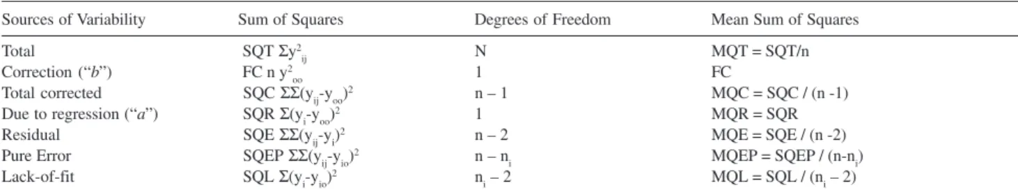
In order to perform the lack-of-fit test, ANOVA statistical test should be carried out. The total variability of the responses is decomposed into the sum of squares due to regression and the residual (about regression) sum of squares and latter is decomposed into lack-of-fit and pure error sums of square. The former is concerned to deviation from linearity and the latter from repeated points. Replications of each calibration point give information about the inherent variability of the response measurements (pure error). If the replicates are repetitions of the same reading or obtained by successive dilutions, the residual variance σ2
res will tend to underestimate the variance σ2 and the lack-of-fit test will tend to wrongly detect non-existence lack-of-fit. ANOVA table can be constructed from equations shown in Table 1.
A significant MQR/MQE ratio confirms that there is regression. If the ratio MQL/MQEP is higher than the
critical level, the linear model appears to be inadequate. A non-significant lack-of-fit indicates that there appears to be no reason to doubt the adequacy of the model and both the pure error and lack-of-fit mean squares can be used as estimates of the variance σ2.
Test of homogeneity of variances
The described linear regression calculation requires each data point in the range has a constant (homogeneous) absolute variation. Inhomogeneity can lead to a higher imprecision and to a higher inaccuracy through possible change in the linear slope. In order to test the homogeneity of variances, replicates of n standard samples of each of the lowest and the highest concentrations of the preliminary range are analyzed separately. The means and the variances, for both set of data, are calculated. The variances of both series of measurements are checked for homogeneity using the F-test. When the test statistic does not exceed the critical value, there is no reason to reject the null hypothesis and believe that there is not a significant difference between the variances. In the case of inhomogeneity of variances or non-linearity, the chosen range must be reduced so as to fulfill these conditions, or more complicated calibration methods must be chosen as the weighted regression equations or higher degree-regression functions.13-16
Experimental
In the present study, FAAS was used for the nickel determination and the uncertainty of the calibration function was assessed. Measurements were obtained by using a Perkin Elmer Flame Atomic Absorption Spectrometer, 5000 Model, with a nickel hollow cathode lamp as the external source, at 232 nm wavelength and 0.2 nm resolution width, and a deuterium lamp as the background corrector. All chemical reagents were analytical grade.
A solution of HNO3 0.1 mol L-1 was prepared for the leaching step. The studied material was a sample of
Table 1. ANOVA table for OLS
Sources of Variability Sum of Squares Degrees of Freedom Mean Sum of Squares
Total SQT Σy2
ij N MQT = SQT/n
Correction (“b”) FC n y2
oo 1 FC
Total corrected SQC ΣΣ(yij-yoo)2 n – 1 MQC = SQC / (n -1) Due to regression (“a”) SQR Σ(yi-yoo)2 1 MQR = SQR
Residual SQE ΣΣ(yij-yi)2 n – 2 MQE = SQE / (n -2)
Pure Error SQEP ΣΣ(yij-yio)2 n – n
i MQEP = SQEP / (n-ni)
Lack-of-fit SQL Σ(yi-yio)2 n
i – 2 MQL = SQL / (ni – 2)
vermiculite containing nickel ions as contaminant. The sample was dried at 60 °C for 2 h to remove water. Adequate aliquots of a NIST certificated standard solution of 1.000 ± 0.002 g L–1 of nickel were diluted with deionised water to obtain five solutions (2.0, 3.0, 4.0 and 5.0 mg L–1) for the calibration function. The nickel responses were measured in acid solutions obtained from leaching 56.3 mg of the solid material with 15 mL of 0.1 mol L-1 HNO
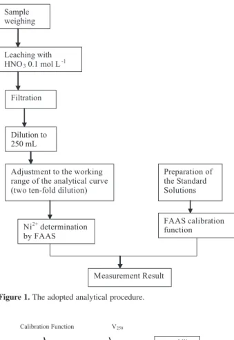
3 solution. After filtration of the leachate through a Whatman medium porosity filter paper, the filtrate was made up to 250 mL in a volumetric flask. Two ten-fold dilutions with deionised water were carried out to adjust nickel concentration to the calibration curve working range. The analytical procedure is illustrated schematically in Figure 1.
Uncertainty components (Figure 2) were quantified for each step of the analytical procedure as follows: weighing operation, dilution effects, measuring nickel ions by flame atomic absorption spectrometry using a linear calibration function, and calculation of the final result.
Results and Discussion
Investigation of the contribution of individual steps
Step 1: weighting
Several sub-samples of 56.3 mg of the dried solid sample were weighted by the difference between container plus sample and container without sample. The uncertainty in the balance certificate was stated as ± 0.1 mg at a 95% confidence level. A standard deviation of 0.0510 was calculated dividing 0.1 by 1.96. The value 0.0510, in equation (3), was multiplied by 2, considering two times weighting (related to container plus sample and container without sample). The run-to-run variability, ± 0.09902 mg, was estimated by means of a Shewhart control graph.19,20 Combining these components the standard uncertainty due to weighting operation in equation (3) resulted in 0.1225 mg:
(3)
Step 2: dilution
The uncertainty of the internal volume of the 250 mL volumetric flask was indicated by the manufacturer as ±0.15 mL.21,22 Since this figure was not given with a confidence level, the appropriate standard deviation was calculated as 0.15: 61/2= 0.0612 mL assuming a triangular distribution.5,6
The effect due to temperature difference, from the moment of the flask calibration until the analysis time, was calculated as ± 3 °C. Since the volume expansion coefficient of the liquid (2.1×10⁻⁴ °C-1 at 20°C) was considerably greater than that of the flask (10×10–6 °C-1 for borosilicate glass flasks), only the former was considered. So, the temperature effect for the dilution step resulted in ± 250 × 3× 2.1×10–4 = ± 0.1575 mL. The standard deviation was calculated as 0.1575:31/2= 0.09094, assuming an approximated rectangular distribution.5 The uncertainty due to the made up to volume step by the operator, expressed as the repeatability run-to-run operation, was ± 0.020 mL.
Combining the three contributions to the uncertainty of the 250 mL volume (V250) the result was:
(4) Figure 1. The adopted analytical procedure.
Two ten-fold dilutions were necessary to adjust the expected level of nickel in the solution to the working range of the analytical curve. Contributions due to repeatability and variation within specification limits were determined and combined for each type of glassware available (10 mL pipettes and 100 mL volumetric flasks). Table 2 summarizes the calculation of the uncertainties from repeatability run-to-run operation and arising from variation within specification limits and temperature difference.
There was an uncertainty associated with the initial and final volumes taken, so the dilution factor uncertainty was associated with them. Dilution factors were calculated as:
(5)
where sfactor10 = the standard deviation of the dilution factor.
Step 3: measuring nickel by Flame Atomic Absorption Spectrometry using a linear calibration function
The calibration experiment was started with the choice of a preliminary linear working range from 1.0 to 5.0 mg L–1 nickel ions. Five analytical solutions (concentrations of 1.0, 2.0, 3.0, 4.0 and 5.0 mg L–1)
were prepared from a 1.000 ± 0.002 g L–1 nickel
solution. The analytical curve was prepared and measured three times in order to estimate day-to-day
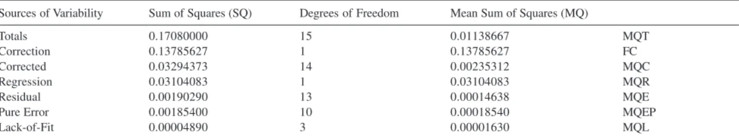
variation. Three replicates of each of the lowest and the highest concentration of the working range were submitted to a linear regression analysis to obtain the coefficients “a” and “b”. Table 3 summarizes the analysis of variance.
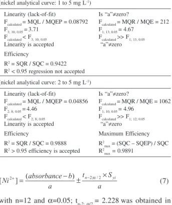
Homogeneity of variances and linearity were verified by a statistical significance test. Table 4 shows the results of linearity and regression efficiency tests.9,10
Looking at Table 4, it was observed that R2 = 0.9422 and R2
max= 0.9437 for the studied concentration range of 1 to 5 mg L-1 ; since R2 > 0.95 was the adopted criterion to accept the regression,9,10 the lowest concentration (1 mg L-1 Ni2+) was eliminated to proceed to a new analyses of variance. For the new range (2 to 5 mg L-1 Ni2+) the tests showed R2 = 0.9888 and R2
max= 0.9891. The calibration function was y = 0.0321667x – 0.0006333, with Sb2= 9.75846×10⁻⁶ e S
a
2= 4.87923×10⁻⁶ as the coefficients variances.
Uncertainty due to variability in “y” was estimated7,9,10,14 by calculating equation (6):
(6)
wherer = number of sample replications, Sb2= MQE/n (contribution due to “b”), n = number of standard solutions (working range), Sa2= MQE / Σ
xx(contribution due to “a”),
Sxx= Σ(xi– xm)2,
xm= Σxi/ n.
The diluted solution, that contained nickel ions originated from the leaching step (one replication, r = 1) resulted in 0.083 of absorbance. Equation (7) provided the amount of nickel present in the diluted solution using the calibration function y = 0.0321667x – 0.0006333:
Table 3. Analysis of variance-nickel analytical curves
Sources of Variability Sum of Squares (SQ) Degrees of Freedom Mean Sum of Squares (MQ)
Totals 0.17080000 15 0.01138667 MQT
Correction 0.13785627 1 0.13785627 FC
Corrected 0.03294373 14 0.00235312 MQC
Regression 0.03104083 1 0.03104083 MQR
Residual 0.00190290 13 0.00014638 MQE
Pure Error 0.00185400 10 0.00018540 MQEP
Lack-of-Fit 0.00004890 3 0.00001630 MQL
Table 2. Uncertainties due to run-to-run operations, manufacturer’s specifications and temperature effect
Volumetric materials s* tolerance/31/2 + combined standard Standard Relative Standard temperature effect deviation Uncert.-1s (mL) Uncert. (1s/V)
10 mL pipette 0.012 0.00894 (0.0122 + 0.008942)1/2 0.0150 0.00150
100 mL flask 0.010 0.0547 (0.0102 + 0.05472)1/2 0.0556 0.000556
250 mL flask 0.020 0.1096 (0.0202 + 0.10962)1/2 0.1114 0.000446
(7)
with n=12 and α=0.05; tn-2; α/2 = 2.228was obtained in statistical tables considering (n-2) degrees of freedom concerning the residual factor.
0321667 . 0
003489 . 0 228 . 2 0321667 . 0
0006333 . 0 083 .
0 ×
± +
) 24 . 0 60 . 2
( ±
] [Ni2+ =
] [Ni2+ =
mg L-1
Due to the calibration function, xobserved = 2.60 mg L-1 and it was associated with the uncertainty of ± 0.24 mg L-1 (in percentage, expressed as ± 9%).
Step 4: calculation of final result
The final result expressed as mg of nickel per mg of solid sample was calculated as 0.046 mg.
Uncertainty of the final result (0.046 mg) was estimated by the combination of the components described in Table 5.
According to the new recommended nomenclature5,6 total uncertainties as combined uncertainty, uc, and expanded uncertainty, U, were calculated:
The final result and uncertainty was (0.046 ± 0.004) mg of nickel per gram of solid sample or expressed as 0.046 mg with associated uncertainty of ± 9%.
Conclusions
It can be observed that the uncertainty due to xobserved is much higher than the other figures. The measured value 2.60 mg L–1 is associated with an uncertainty of ± 0.24 mg L–1, due to the function calibration. This figure represents an uncertainty of ± 9% (= 0.23:2.60×100 ± 9%). The final result for the nickel determination resulted in 0.046 mg with an expanded uncertainty of ± 0.004. In percentage, this also represents ± 9% (= 0.004:0.046×100). Hence, the uncertainty estimate of the various steps of an analysis demonstrates that the calibration step might give an important contribution to the uncertainty of the final result. In the present case, it is the main factor.
Analysts should pay more attention to the experiment planning of the analytical curve, in order to obtain lower limits for uncertainty when linear least squares fit is considered. They should take into account the verification of linearity, the test of homogeneity of variances and the confirmation of regression efficiency. And not just using the linear least squares fit procedure, assuming that the calibration is properly performed by calculating the correlation coefficient R when this figure is close to –1 or +1. Finally, the ordinary linear regression validity should be demonstrated and the uncertainties of linearity, slope and ordinate intercept estimated.
Preparing replicates of known concentration solutions is an important condition to the assessment of uncertainties estimates for the calibration curve. By carrying out more replicates of solutions with known concentrations to build the calibration curve itself, one can increase the number of degrees of freedom using lower values for the statistic “t” and, in consequence, obtaining lower limits of uncertainties. Analyzing more replicates of samples will also help to decrease uncertainty of the final result.
Table 5. Intermediate values and uncertainties for nickel determination Sources of Value (v) Standard Relative Standard Uncertainties Uncertainty (1s) Uncertainty (1s/v) xobs/(mg L-1) 2.60 0.108466a 0.0417177 final Vf /(mL) 250 0.1114 0.0004384 dilution factor 2 × 10b 0.02263b 0.0002263 Initial mass/(mg) 56.3 0.1225 0.002176 aFigure calculated Sy
I / a = 0.003489/0.0321667 = 0.108466;
bExpressed by two ten-fold dilution; .
Table 4. Results of linearity and regression efficiency tests (nickel analytical curve: 1 to 5 mg L-1)
Linearity (lack-of-fit) Is “a”≠zero?
Fcalculated = MQL / MQEP = 0.08792 Fcalculated = MQR / MQE = 212 F3; 10; 0.05 =3.71 F1; 13; 0.05 = 4.67
Fcalculated < F3; 10; 0.05 Fcalculated >> F1; 13; 0.05 Linearity is accepted “a”≠zero Efficiency
R2 = SQR / SQC = 0.9422 R2 < 0.95 regression not accepted (nickel analytical curve: 2 to 5 mg L-1)
Linearity (lack-of-fit) Is “a”≠zero?
Fcalculated = MQL / MQEP = 0.04856 Fcalculated = MQR / MQE = 1062 F2; 8; 0.05 =4.46 F1; 10; 0.05 = 4.96
Fcalculated < F2; 8; 0.05 Fcalculated >> F1; 12; 0.05 Linearity is accepted “a”≠zero
Efficiency Maximum Efficiency
R2 = SQR / SQC = 0.9888 R2
max = (SQC – SQEP) / SQC R2 > 0.95 efficiency is accepted R2
In cases when the OLS regression validity cannot be demonstrated, others techniques should be used such as the weighted regression equations or higher degree-regression functions.
Supplementary Information
Supplementary data are available free of charge at http://jbcs.sbq.org.br, as PDF file.
References
1. http://www.cetesb.sp.gov.br/Solo/solo_geral.asp, acessed in September 2006.
2. ISO (1990) Accuracy (trueness and precision) of measurement methods and results. Part I – General principles and definitions (ISO-DIS 5725/1990). International Organization for Standardization, Geneva.
3. Buchmann, J.H.; Sarkis, J.E.S.; Quim. Nova2002, 25, 111. 4. Horwitz, W.; Albert, R.; Analyst1997, 122, 615.
5. EURACHEM (1999) Working Group Quantifying Uncertainty in Analytical Measurement, English 2nd ed. Draft EURACHEM/ CITAL (English 1st ed. Crown Copyright, London).
6. ISO (1995) Guide to the expression of uncertainty in measurement. International Organization for Standardization, Geneva (ISO GUM).
7. Otto, M.; Chemometrics-Statistics and Computer Application in Analytical Chemistry, 1st ed., Wiley-VCH: New York, 2000, ch.5.
8. Draper, N.R.; Smith, H.; Applied Regression Analysis, Wiley: NewYork, 1998.
9. Waeny, J.C.C.; Comunicação Técnica 12: Aplicações metrológicas da regressão-II Análise da variância, IPT, 1983, São Paulo, Brasil, p. 41.
10. Giller, M.; Specialisation course in Quality Engineering. Parana Catholic University, Curitiba, Brazil, 1994, p. 65.
11. RSC-Royal Society of Chemistry/Analytical Methods Committee; Analyst1988, 113, 1469.
12. RSC-Royal Society of Chemistry/Analytical Methods Committee; Analyst1994, 119, 2363.
13. Mandel, J; J. Qual. Technol.1984, 16, 1.
14. Werner F.; Dammann, V.; Donnevert, G.; Quality Assurance in Analytical Chemistry, VCH Publishers: New York, USA, 1995. 15. Barros Neto, B.; Pimentel, M.F.; Araújo, M.C.U.; Quim. Nova
2002, 25, 856.
16. Burdge, J.R.; MacTaggart, D.L.; Farwell, S.O.; J. Chem. Ed. 1999, 76, 434.
17. Ferreira, M.M.C.; Antunes, A.M.; Melgo, M.S.; Volpe, P.L.O.;
Quim. Nova 1999, 22, 724.
18. Dantas Filho, H.A.; Souza, E.S.O.N.; Visani, V.; Barros, S.S.R.C.; Saldanha, T.C.B.; Araújo, M.C.U.; Galvão, R.K.H.;
J. Braz. Chem. Soc.2005, 16, 58. 19. Mullins E.; Analyst1994, 119, 369.
20. BSI (1984) British Standard Guide to process control using quality control chart method and cusum techniques. British Standard International, London (BS 5700/1984).
21. ISO (1968) One mark volumetric flasks. International Organization for Standardization, Geneva (ISO-TC48-R1042/ 1968).
22. ISO (1976) Laboratory glassware, one mark pipettes. International Organization for Standardization, Geneva (ISO-DIS 648/1976).
Received: July 13, 2006
Web Release Date: April 11, 2007