www.geosci-model-dev.net/9/789/2016/ doi:10.5194/gmd-9-789-2016
© Author(s) 2016. CC Attribution 3.0 License.
IL-GLOBO (1.0) – development and verification of the moist
convection module
Daniele Rossi, Alberto Maurizi, and Maurizio Fantini
Institute of Atmospheric Sciences and Climate, National Research Council, CNR-ISAC, Bologna, Italy Correspondence to:Alberto Maurizi ([email protected])
Received: 3 August 2015 – Published in Geosci. Model Dev. Discuss.: 28 September 2015 Revised: 16 February 2016 – Accepted: 19 February 2016 – Published: 26 February 2016
Abstract. The development and verification of the convec-tive module of IL-GLOBO, a Lagrangian transport model coupled online with the Eulerian general circulation model GLOBO, is described. The online-coupling promotes the full consistency between the Eulerian and the Lagrangian com-ponents of the model. The Lagrangian convective scheme is based on the Kain–Fritsch convective parametrization used in GLOBO. A transition probability matrix is computed us-ing the fluxes provided by the Eulerian KF parametrization. Then, the convective redistribution of Lagrangian particles is implemented via a Monte Carlo scheme. The formal deriva-tion is described in details and, consistently with the Eule-rian module, includes the environmental flux in the transition probability matrix to avoid splitting of the convection and subsidence processes. Consistency of the Lagrangian imple-mentation with its Eulerian counterpart is verified by com-puting environment fluxes from the transition probability ma-trix and comparing them to those computed by the Eulerian module. Assessment of the impact of the module is made for different latitudinal belts, showing that the major impact is found in the Tropics, as expected. Concerning vertical distri-bution, the major impact is observed in the boundary layer at every latitude, while in the tropical area, the influence ex-tends to very high levels.
1 Introduction
Long-range transport of atmospheric tracers plays an impor-tant role in several fields ranging from atmospheric composi-tion and chemistry to climate change, with applicacomposi-tions span-ning from air pollution to natural or anthropogenic disaster management and assessment.
Lagrangian description is the natural framework for tracer dispersion modelling, and the use of Lagrangian particle dispersion models (LPDM) for both theory and application is very effective and widespread. In particular, Lagrangian models are used often to retrieve information about the sources contributing to the concentration at a specific lo-cation (known as “backtrajectories”). The consistent imple-mentation of LPDM requires the careful consideration of all the processes involved in the atmospheric dispersion.
Depending on the geographical area and season, the re-distribution of tracers released in the atmosphere can be largely affected by the vertical transport due to moist con-vection events. In particular, concon-vection is very efficient in mixing the boundary layer with the free-troposphere air (Cot-ton et al., 1995) contributing to the long-range spread of local emissions.
Moist convection is widespread in the Earth’s atmosphere where it displays a wide range of space- and timescales in re-sponse to the variability of environmental parameters, rang-ing from the sub-kilometre/tens-of-minutes of individual cu-muli to hundred-of-kilometre/several days of mesoscale con-vective complexes (see e.g. Emanuel, 1994).
For all the scales smaller than or close to the grid size of the numerical models, explicit resolution is inadvisable, and numerical models resort to parametrization schemes.
For the turbulent diffusion processes (that are predominant in the boundary layer), whose typical space- and timescales are small compared to the resolution of a general circula-tion model, a well-founded theoretical framework exists and allows for the formulation in terms of stochastic processes (Thomson, 1987). In contrast, mass-flux theories of moist convection do not provide sufficient details to implement stochastic models. Therefore, moist convection effects are simulated using particle redistribution mechanisms, which reproduces the expected mass fluxes obtained from an Eule-rian convective scheme parametrization, usually via a Monte Carlo scheme (e.g. Forster et al., 2007).
While coupled chemistry and meteorology models (CCMMs) are now at the front edge of research in atmo-spheric composition studies (Baklanov et al., 2014), popu-lar LPDMs are designed for offline usage and need to re-construct necessary quantities that are not included in the normal output of meteorological models. In particular, off-line recalculation of convective mass fluxes is needed, from quantities made available from the meteorological (Eulerian) model such as temperature and moisture, and is often per-formed with a mass-flux scheme different from the one that produces the meteorological output (see e.g. Forster et al., 2007), possibly leading to dynamical inconsistencies in the results.
To avoid this inconsistency, IL-GLOBO (Rossi and Mau-rizi, 2014) was designed as an online-coupled model that makes use of the full availability of Eulerian fields. In its first step of development, the vertical transport and disper-sion of tracers were the result of the vertical advection and diffusion only. In the absence of a convective parametriza-tion, explicit convection can occur, and thus some verti-cal transport of tracers were present in the previous ver-sion of the model. However, since the scales of convection are in the sub-kilometre range, any explicit representation of it at coarser resolution is bound to misrepresent most of those scales, and create updrafts that are incorrect in loca-tion and strength. Therefore the inclusion of a moist con-vection Lagrangian redistribution mechanism is essential to the completeness of the model. The IL-GLOBO moist con-vection module is developed consistently with the modified KF scheme adopted in GLOBO (Malguzzi et al., 2011) (see Sect. 2). With the online coupling this module benefits from the full availability of all meteorological variables at every time step.
In this paper the development of the online-coupled con-vective module of IL-GLOBO is presented and its features will be assessed through some application examples. In Sect. 2 the Eulerian convective parametrization is presented while the implementation of the Lagrangian scheme is de-scribed in Sect. 3 with emphasis on Eulerian consistency and providing full details of the constructive procedure. Verifica-tion of the scheme and some evaluaVerifica-tion of the inclusion of convective effects in IL-GLOBO are presented in Sect. 4.
2 The Kain–Fritsch scheme
A convective parametrization that makes explicit use of the vertical fluxes of mass, the KF scheme, was adopted by the GLOBO developers, and in the present work, for its ready availability, ease of implementation and widespread use by the meteorological research community.
The original formulation, and its successive evolution, were presented in a series of papers (Fritsch and Chappel, 1980; Kain and Fritsch, 1990; Kain, 2004) to which the reader is referred for more details. Recent presentations of its performance in the simulation of meteorological events can be found e.g. in Liu and Wang (2011) and Bullock et al. (2015).
The scheme is based on a steady-state entraining– detraining plume model and a closure based on release of convective available potential energy (CAPE). Three streams of mass are present: updraft and downdraft of the convecting ensemble, and a weak environmental flow (subsidence) that maintains the balance of mass at each model level.
The updraft is a detailed account of the thermodynamics of moist air and entrainment–detrainment of moisture and condensate at every level between cloud base and the cloud top. Briefly, mixtures of low-level air are tested for instabil-ity. Once a lifted condensation level (LCL) is identified, the parcel buoyancy at each upward level is computed, and an es-timate of the kinetic energy gained by latent heat release ob-tained. The, as yet unspecified, upward mass flux is then frac-tionally increased/reduced by entrainment/detrainment of en-vironmental air based on a buoyancy-sorting principle. The dilution of the originally unstable air with drier and cooler air from the environment reduces its buoyancy, up to an equilib-rium level (LET) where the rising air has no more accelera-tion from thermodynamic processes. Upward of the LET, the rising air is decelerated until the remaining kinetic energy of the vertical motion is reduced to zero, which defines the top of the cloud.
Downdrafts are generated by re-evaporation of water con-densate expelled by the rising motion. Environmental air is assumed to be entrained uniformly into the downdraft in a layer around cloud base, and detrained, again linearly in pres-sure, at lower levels. The empirical evidence for this structure is discussed at length in Kain (2004).
Only at this point are the dimensional mass fluxes deter-mined by applying the closure assumption that requires at least 90 % of the CAPE to be consumed by the ensemble of convective clouds. This finally determines the fraction of a grid box covered by the ensemble of clouds and the environ-mental subsidence needed to maintain the balance of mass at each level.
The tendencies of thermodynamic quantities to be returned to the model are spread over a “convective timescale”1TC,
Cloud top
Cloud base
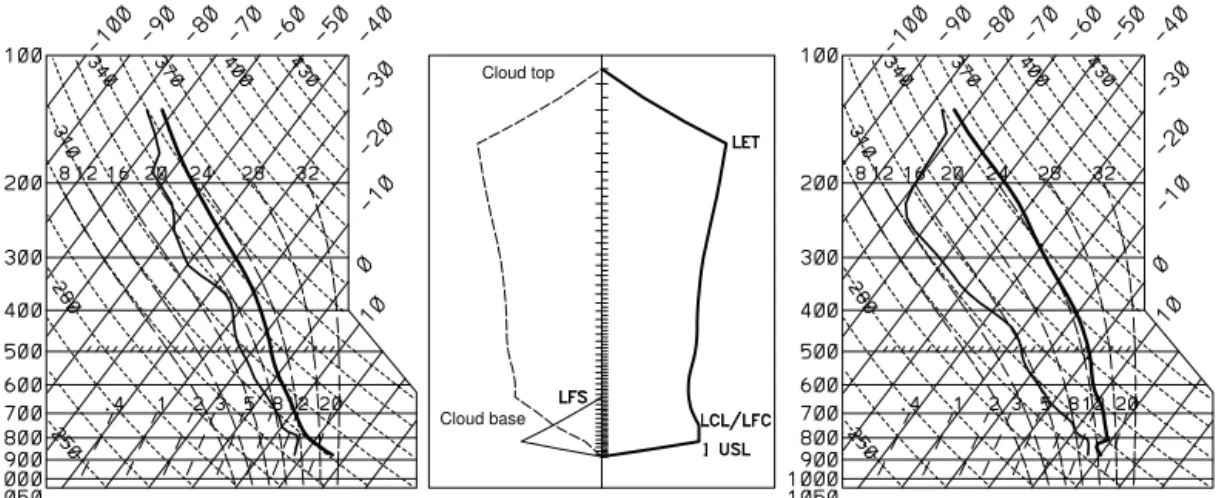
Figure 1.SkewT–logP thermodynamic diagrams for a deep tropical convective episode, before (left panel) and after (right panel) the action of convection as determined by the parametrization scheme: pressure on left axis in hPa, temperature on right and top axes in◦C. Middle panel: profiles of vertical mass fluxes as computed by the convection scheme: updraft (Fu, thick solid line), downdraft (Fd, thin solid line), environmental subsidence (Fe, dashed) needed to maintain the balance of mass at each level (see Fig. 2 for definitions). Vertical coordinate for the middle panel is pressure, with the same scale indicated for left and right panels. Horizontal coordinate is kg s−1m−2with arbitrary scale: the flux per unit area depends on the area attributed to the convective ensemble by the convection scheme. In this instance it is about 7 % of the grid box. Also shown on the central axis are the locations of model levels. Significant levels for the convection computation are labelled on the graph. The air in the updraft source layer (USL) becomes saturated when raised to the lifted condensation level (LCL), and is unstable when further pushed to its level of free convection (LFC – at the same model level in this instance). Vertical acceleration of the rising air parcel ceases at the level of equilibrium temperature (LET) and vertical motion stops at cloud top. The convective downdraft begins at the level of free sink (LFS) and extends down to the ground.
An example of the effect of the scheme on an unstable atmospheric profile is shown in Fig. 1.
3 Lagrangian implementation of the moist convection effects
IL-GLOBO uses some of the quantities computed by the KF convective parametrization (see Sect. 2) to implement a Monte Carlo scheme (KF-MC) for the particle displace-ment, in a way similar to other LPDMs (Collins et al., 2002; Forster et al., 2007). All these schemes compute the displace-ment probability matrix (DPM) between levels making use of the entrainment and detrainment fluxes in updraft and down-draft. Additionally, in IL-GLOBO the environment effects (subsidence), that result from a mass balance, are directly included into the DPM, and therefore implemented using the MC scheme, without the need of a posteriori adjustment.
In the following, the same notation as in Fig. 1 of Rossi and Maurizi (2014) is used where NLEVσ-hybrid grid levels are indexed decreasing with height.
In the Eulerian model component, every1TC(or, in terms
of time steps, every nC advective time step 1t), the KF
scheme checks for the conditions for the onset of convection and, if conditions are met, determines the evolution of the grid column for the whole 1TC. Entrainment and
detrain-ment fluxes in both updraft (fuε,fuδ) and downdraft (fdε,
fdδ) for each level (see Fig. 2), from the ground to the cloud
Fui Fei Fdi
Fui+1 Fei+1 Fdi+1
fuiε fdiδ
fuiδ fd ε i
Updraft Environment Downdraft
i+1
i−1
i
i+1 i
Figure 2.Schematic representation of fluxes involved in the KF scheme. UppercaseF represent the fluxes between vertical levels (across level boundaries) while lowercasef are the fluxes within a level that represent the exchange of mass between environment (e) and updraft (u) or downdraft (d), respectively.
top, as computed by the KF scheme are made available to the Lagrangian model. With reference to Fig. 2, the following relationships hold for fluxes at (f) and between (F) levels:
Fiu=Fiu+1+fiuε−fiuδ (1) for the updraft (u) and
(fiuε1t /mei) and the probability that the particle resides in the environment (mei/mi), where mei is the mass already
present in the environment as opposed to the mass flowing through, in the convective ensemble, andmi is the total mass
of the leveli, giving
puiε=f uε i 1t
mi
. (3)
The probability that a particle captured by the updraft is de-trained can be easily derived by rearranging Eq. (1) into
Fiu
Fiu+1+fiuε + fiuδ
Fiu+1+fiuε =1. (4)
Noticing that the two terms are both positive by definition, the above relationship can be used to define the probability
puiδ= f uδ i
Fiu+1+fiuε, (5)
which is identically equal to 1 at the cloud top whereFiu top=
0. The denominatorFiu+1+fiuεof Eq. (4) is the flow entering the updraft volume (see Fig. 2) at leveliand that is available to detrainment process. The mass entering the leveliwhich is not detrained must flow to the upper level satisfying the continuity for the updraft (Eq. 1). In terms of probability, this is expressed by the complementary probabilitypiuδ=1−puiδ
puiδ= F u
i
Fiu+1+fiuε (6)
which, combined with Eq. (5), gives back Eq. (1) confirm-ing the consistency of the above definitions of the probability components.
Using the above definitions it is possible to build the full transition probability matrix for the updraft fraction. The probability that a particle moves due to the updraft motion from a levelito a levelj < iis equal to the probability that the particle is entrained at leveli(Eq. 3) times the probabil-ity that it is detrained at levelj (Eq. 5) times the probability that it is not detrained between leveliandj+1 included. In formula:
pu(j|i)=piuεpjuδ
j+1
Y
k=i
1−pukδ
. (7)
For the downdraft transition probability pd, a similar rela-tionship holds. The probabilitiespuandpdrepresent the up-per and lower triangular components of the total convective transition probability matrixpcwhose diagonal is defined by pc(i|i)=1−p1uε 1−puiδ
−pdiε 1−pdiδ. (8)
The mixing produced by the convective motion (updraft and downdraft) needs to be balanced by the environment flux (subsidence) to conserve the mass. For the Eulerian part this is granted by the environmental flux computed in the KF scheme. In Lagrangian terms this is equivalent to maintain-ing a well-mixed state where the redistribution of mass is applied, and can be expressed in terms of DPM. This con-sistency is obtained by modifying the transition probability matrixpcby imposing zero net flux at the interface between two model levels. At leveli, the mass fluxes (assumed posi-tive upward) across the two level interfacesi(upper) andi+1 (lower) due to the sum of updraft and downdraft motion, are expressed in terms of probability as
Fic=X k<i
pc(k|i) mi−pc(i|k) mk (9)
and
Fic+1=X k>i
pc(i|k) mk−pc(k|i) mi (10)
respectively. Thus, the mass conservation reads
Fic+Fie=Fic+1+Fie+1, (11) whereFe is the environment mass flux which is directed downward except in very peculiar cases (Kain et al., 2003)1. With the additional boundary condition
FNLEVe +1=0, (12)
the environment flux can be computed iteratively through Eqs. (9)–(11). The effect of the environment flux at surface
i+1 is to increase the transition probability fromitoi+1 while reducing the probability of the “null transition” (par-ticle remains in the same model level). This results in the modification of the elements of the diagonal:
p(i|i)=pc(i|i)−F e
i+11t mi
(13) and sub-diagonal:
p(i+1|i)=pc(i+1|i)+F e
i+11t mi
. (14)
The final DPM is then defined by
p(j|i)≡pc(j|i) (15)
forj < iorj > i+1 and by Eqs. (13) and (14) forj =iand
j=i+1, respectively.
It is worth noting thatp is an Eulerian quantity that can be viewed as the linear operator acting on an initial concen-tration vector to give the concenconcen-tration distribution after the
1The very unlike case of upwardFeis accounted for in the
convection mixing. However, sincepis defined in terms of a finite time step1t, it may become unstable (flux in one time step comparable to or larger than the mass of the level). In fact, KF use a reduced time step1tKF=1TC/nKF, with
in-tegernKF, internally computed to maintain linear stability of
the numerical scheme. Consistently, the same1tKF is used
to compute the transition probability that will be iteratednKF
times using the MC scheme.
In order to implement the MC scheme, it is convenient to compute the cumulative transition probability matrixPas
Pj,i= j
X
k=NLEV
p(k|i) . (16)
The MC scheme is applied in grid columns affected by con-vection to the particles that are below the cloud top by ex-tracting a random numberχ, uniformly distributed between 0 and 1, and comparing its value toPj,i, j=NLEV, itopuntil
ajf is found so thatχ <Pjf,i. A position is then attributed
to the particle within the arrival grid cell using the same χ
number to interpolate linearly between the grid cell bound-aries (Forster et al., 2007):
σp=σ (jf)+ χ−Pjf−1,i
/ Pjf,i−Pjf−1,i
1σ . (17) The MC scheme is iteratednKFtimes to obtain the final
posi-tion after1TC. Then, as for the tendencies of thermodynamic
quantities in the Eulerian part, the total particle displacement is spread over thenCadvective time steps that cover the
con-vective period.
4 Model verification
In order to identify the main features of the KF-MC scheme, to verify its implementation and to assess its impact on dis-persion, some numerical experiments were performed.
A number of convective episodes were extracted from a model simulation performed using a horizontal regular grid of 1200×832 cells of 0.3◦×0.22◦, that corresponds to a res-olution of about 23 km at mid-latitudes in longitude, and a regular vertical grid of 50 points in theσ-hybrid coordinate. The advective time step used was 1t=150 s. The convec-tive timescale isTC≃30 min, i.e. the KF scheme is executed
everynC=11 advective time steps.
4.1 Displacement probability matrix
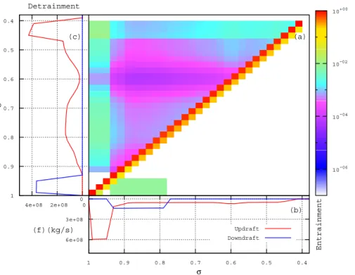
An example selected in the tropical area around noon is shown in Fig. 3. The central part of the figure show the DPM for that specific event along with the vertical profiles of entrainment (bottom) and detrainment (left) fluxes in both updraft and downdraft. In this example the significant lev-els as defined in Fig. 1 are σcloud top=0.41, σLET=0.47, σLFS=0.79,σLCL=0.93 and the USL is a mixture 60 hPa thick based on the ground. The two most likely transitions are:
1. the particle stays within the starting grid cell (highest values are found in the diagonal because most of the model grid cell is not influenced by convection); 2. the particle is transferred in the cell just below, due to
the environment flux (high values in the matrix sub-diagonal).
The other transitions are directly caused by convective mo-tion and are consistently less likely, with probabilities in the range 10−2–10−5. It is expected that finer model reso-lution would increase the ratio between the volume involved in convection to the total volume of some model columns. Updrafts generate transitions with highest likelihood for dis-placements from levels next to the ground to levels just below the cloud top, while the downdraft transitions are permitted only from levels between 0.8 and 0.9σ to levels between 0.9 and 1.0σ. This reflects the hypotheses underlying the formu-lation of the KF parametrization.
4.2 Algorithm verification
In order to verify the consistency of the implementation, the distribution of initially well mixed particles were verified af-ter convection to be still well mixed. This is performed in 1-D-like configuration by selecting 12 convectively active grid columns, releasing 4×10⁴well-mixed particles in each and integrating the model for a full1TC. It is found that the
dis-tribution after such integration remains well mixed within the same error interval used in Rossi and Maurizi (2014). However, this only provides a test of the numerical imple-mentation and not of the theoretical formulation and correct calculation ofpc. In fact, in contrast to the formulation of a Lagrangian turbulent diffusion model for which well mix-ing provides a necessary and sufficient condition (Thomson, 1987), the well-mixed state in the present scheme is main-tained by construction of the environmental flux, whether pcis correct or not. Therefore an independent verification is necessary. This is done by comparing the environment fluxes computed using the DPM from Eqs. (9), (10) and (11) to those provided by the KF scheme. Such a verification, per-formed for a number of convective episodes, confirms that within the roundoff error (10−7) Eulerian and Lagrangian KF fluxes are the same.
4.3 Impact of KF-MC on dispersion
The impact of convection on the particle dispersion in a fully 3-D experiment is considered. The aim is to assess the im-portance of the moist convection mechanism with respect to diffusion and advection. Simulations start on 11 March 2011. Particles are released and then dispersed for 6 days, and their position is sampled every hour. The source con-sists of Np≃7.4×10⁵ pairs of particles, each pair
shar-ing the same initial position. Particles are released between
0.4
0.5
0.6
0.7
0.8
0.9
1
0 2e+08 4e+08
σ
Detrainment
10 06 1004 10___––_––02 10+00
0
3e+08
6e+08
0.4 0.5 0.6 0.7 0.8 0.9 1
Entrainment
σ
Updraft Downdraft
(f)(kg/s)
(a)
(b) (c)
-Figure 3.Example of Displacement Probability Matrix (DPM) and the fluxes generated by the convection mechanism, as function of the vertical σ-hybrid coordinate. Panel(a)displays the DPM with origins of displacement in the abscissa and destination in the ordinate. Bottom(b)and left(c)panels display entrainment and detrainment fluxes, respectively, for both updraft (red) and downdraft (blue).
density profile, and homogeneously distributed in the hori-zontal within three zonal areas: around the Equator, within the tropical area (−15◦,+15◦), and at mid-latitudes in the Northern Hemisphere and (+30◦,+60◦) and Southern Hemi-sphere (−30◦,−60◦). For each emission area, two different simulations were performed with the KF-MC switched on and off. Values of relative and absolute dispersion are shown in Fig. 4. Absolute dispersion is computed as
12a= 1
2Np
2Np
X
p=1
xp−xp02, (18)
where xp is a generic particle coordinate that can indicate both the particle vertical position (in Fig. 4 represented as the height above the model surface) and the horizontal dis-tance along the Earth surface, andxp0is the starting position of the same particle. Relative dispersion is computed consid-ering the ensemble of pair of particles sharing the same initial position and is defined as
6r2= 1 Np
Np
X
p=1
D
xp1−xp2 2E
, (19)
wherexp1andxp2are the position of each particle of the pair.
Results of the experiments, reported in Fig. 4, show that absolute dispersion is influenced by convection mainly at the Tropics, where the convective activity is more intense and
the tropopause higher. Moreover, the effect is far more rele-vant on the vertical which is the direction directly influenced by the scheme. Concerning the relative dispersion, the moist convection scheme has a relevant impact on both the vertical and horizontal directions. The effect is important in all of the zonal areas but is still more pronounced at the Tropics. The larger impact on horizontal relative dispersion compared to the absolute dispersion can be explained by considering that as particles separate due to convection, they are captured by different horizontal structures that, in turn, rapidly decorre-late the motion of the two particles of the pair.
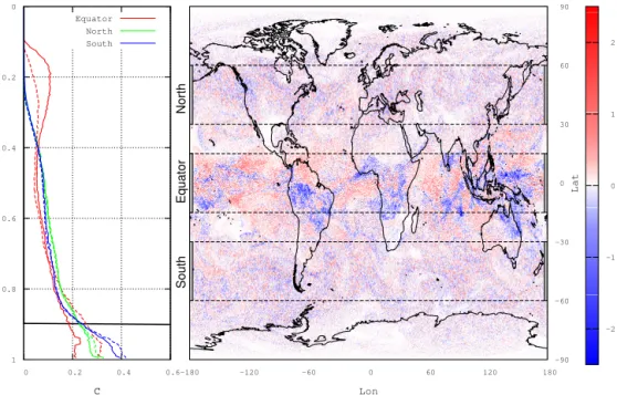
The effect on concentration is shown in Fig. 5, where the final concentration is displayed for vertical (Fig. 5, left panel) with and without moist convection scheme. For the hori-zontal Fig. 5, right panel, a difference map is shown. Parti-cles were counted for intervals of equal size and normalized so that the starting concentration between 0.9 and 1.0σ is around 1. Figure 5, left panel shows that moist convection has an important effect close to the surface in all the areas, with an enhanced effect at the Tropics. In the free troposphere, the effect is almost negligible except for the tropical area above
σ=0.4 where the largest effect is observed. It is worth not-ing that, in the tropical area, particles reach high levels even in the simulation without convection although with a concen-tration smaller by a factor of 2. Since the diffusivity only acts between 0.8 and 1σin the vast majority of cases, the vertical transport of particles producing the high concentration above
0 1000 2000 3000 4000 5000 6000 7000
∆
(m)
Absolute
(a)
Vertical
Relative
(b)
0 1000 2000 3000 4000
0 1 2 3 4 5
∆
(km)
Time (days) (c)
0 1 2 3 4 5
Horizontal
Time (days) (d)
Equator North South
Figure 4.Vertical absolute dispersion(a), vertical relative dispersion(b), horizontal absolute dispersion(c), horizontal relative dispersion(d). Notice that panels(b)and(d)share the sameyaxis with panels(a)and(c), respectively. Continuous lines refer to experiments with the MC convection scheme active, while the dashed lines mark experiments made without it. Line colours indicate the tropical distribution (red), northern middle-latitude distribution (green), southern middle-latitude (blue), respectively. Absolute and relative dispersion are defined by Eqs. (18) and (19).
0
0.2
0.4
0.6
0.8
1
0 0.2 0.4 0.6
σ
C Equator
North
South
–180 –120 –60 0 60 120 180
–90 –60 –30 0 30 60 90
Lat
Lon
–2 –1 0 1 2
North
Equator
South
results from large-scale convergence with minor contribution from horizontal advection and orographic effects.
Figure 5, right panel, displays the map of differences of the vertically integrated number of particles between simulations with and without Lagrangian convection scheme. Particles are sampled for each 0.6◦×0.43◦column and the difference is normalized with respect to the initial number of particles per bin. For the case of release in the tropical area, it can be noted that areas of strong depletion are surrounded by rel-atively larger areas where the difference is weakly positive. The structure of convective updrafts (see e.g. Fig. 1) is such that most of the upward-moving mass comes from the lowest levels of the atmosphere (below cloud base) and is returned to the environment in the upper troposphere, in the strong outflow at the top of the cloud, while areas of weak subsi-dence surround the updrafts. Particles released in the extra-tropical regions (north and south) display different qualita-tive behaviour showing smaller-scale features with respect to those released at the Tropics, in agreement with the expected horizontal scales of convective cells.
5 Conclusions
A Lagrangian transport scheme for moist convection is im-plemented online in IL-GLOBO in parallel with the integra-tion of the Eulerian model. This gives the Lagrangian scheme direct access to all the prognostic variables without any need for additional diagnostics and ensures full consistency of the DPM with the parametrization scheme. As a consequence, the Lagrangian and Eulerian descriptions of tracer dispersion in the coupled model are equivalent, as is expected on theo-retical grounds.
This aspect differs from the approach of other mod-els found in the literature. The quantities used in those cases to advect and diffuse Lagrangian particles are diag-nosed from the meteorological thermodynamics profiles with parametrizations that may differ from that of the meteoro-logical model, making the Eulerian–Lagrangian consistency hard to realize.
The consistency of the present scheme with the Eulerian quantities has been verified in a number of offline 1-D tests, where the model is shown to conserve the mass and repro-duce the expected fluxes.
Global experiments with tracers released close to the sur-face at different latitudes show that the effects of the MC-KM is strong and gives rise to large departures from the non-convective version even at mid-latitudes. Vertical distribution displays again a larger difference at the Tropics. However, even with the KF-MC deactivated (but still activated in the Eulerian part, so generating the “correct” dynamics), at the Tropics some tracer is observed to reach very high altitudes. This is found to be a combined effect of advection, both ver-tical and horizontal.
The next step of the IL-GLOBO development will be the validation of the models against available data, for which ap-propriate data sets are scarce, as noted by e.g. Forster et al. (2007).
Code availability
The numerical code of the IL-GLOBO vertical moist con-vection module (Fortran 90) is released under the GPL and is available at the BOLCHEM website (http://bolchem.isac. cnr.it/source_code.do).
The software is packed as a library using autoconf, automakeandlibtoolwhich allows for configuration and installation in a variety of systems. The code is devel-oped in a modular way, permitting the easy improvement of physical and numerical schemes.
The GLOBO model is available upon the signature of an agreement with the CNR-ISAC Dynamic Meteorology Group (contact: [email protected]).
Acknowledgements. The authors would like to thank Piero
Mal-guzzi for making the GLOBO model available and for making himself available for the explanation of the finer points of the numerics. The software used for the production of this paper (model development, model run, data analysis, graphics, type-setting) is free software. The authors would like to thank the whole free software community and, in particular, the Free Software Foundation (http://www.fsf.org) and the Debian Project (http://www.debian.org).
Edited by: O. Boucher
References
Arakawa, A.: The cumulus parameterization problem: Past, present and future, J. Climate, 17, 2493–2525, 2004.
Baklanov, A., Schlünzen, K., Suppan, P., Baldasano, J., Brunner, D., Aksoyoglu, S., Carmichael, G., Douros, J., Flemming, J., Forkel, R., Galmarini, S., Gauss, M., Grell, G., Hirtl, M., Joffre, S., Jorba, O., Kaas, E., Kaasik, M., Kallos, G., Kong, X., Ko-rsholm, U., Kurganskiy, A., Kushta, J., Lohmann, U., Mahura, A., Manders-Groot, A., Maurizi, A., Moussiopoulos, N., Rao, S. T., Savage, N., Seigneur, C., Sokhi, R. S., Solazzo, E., Solomos, S., Sørensen, B., Tsegas, G., Vignati, E., Vogel, B., and Zhang, Y.: Online coupled regional meteorology chemistry models in Europe: current status and prospects, Atmos. Chem. Phys., 14, 317–398, doi:10.5194/acp-14-317-2014, 2014.
Bullock, O. R. j., Alapaty, K., and Herwehe, J. A.: A dynamically computed convective time scale for the Kain–Fritsch convective parameterization scheme, Mon. Weather Rev., 143, 2105–2120, doi:10.1175/MWR-D-14-00251.1, 2015.
Cotton, W. R., Alexander, G. D., Hertenstein, R., Walko, R. L., McAnelly, R. L., and Nicholls, M.: Cloud venting – A review and some new global annual estimates, Earth Science Review, 39, 169–206, 1995.
Emanuel, K. A.: Atmospheric Convection, Oxford Univ. Press, New York Oxford, USA, 1994.
Forster, C., Stohl, A., and Seibert, P.: Parameterization of Convec-tive Transport in a Lagrangian Particle Dispersion Model and Its Evaluation, J. Appl. Meteorol. Clim., 46, 403–422, 2007. Fritsch, J. M. and Chappel, C. F.: Numerical prediction of
convec-tively driven mesoscale pressure systems. Part I: convective pa-rameterization., J. Atmos. Sci., 37, 1722–1733, 1980.
Kain, J. S.: The Kain–Fritsch Convective Parameterization: An Up-date, J. Appl. Meteorol., 43, 170–181, 2004.
Kain, J. S. and Fritsch, J. M.: A one-dimensional entraining-detraining plume model and its application in convective param-eterization, J. Atmos. Sci., 47, 2784–2802, 1990.
Kain, J. S., Baldwin, M. E., and Weiss, S. J.: Parameterized Up-draft Mass Flux as a Predictor of Convective Intensity, Weather Forecast., 18, 106–116, 2003.
Liu, H. and Wang, B.: Sensitivity of regional climate simula-tions of the summer 1998 extreme rainfall to convective pa-rameterization schemes, Meteorol. Atmos. Phys., 114, 1–15, doi:10.1007/s00703-011-0143-y, 2011.
Malguzzi, P., Buzzi, A., and Drofa, O.: The Meteorological Global Model GLOBO at the ISAC-CNR of Italy Assessment of 1.5 Yr of Experimental Use for Medium-Range Weather Fore-casts, Weather Forecast., 26, 1045–1055, doi:10.1175/WAF-D-11-00027.1, 2011.
Rossi, D. and Maurizi, A.: IL-GLOBO (1.0) – integrated La-grangian particle model and Eulerian general circulation model GLOBO: development of the vertical diffusion module, Geosci. Model Dev., 7, 2181–2191, doi:10.5194/gmd-7-2181-2014, 2014.