AN ANALYSIS OF THE IMPORTANCE OF APPROPRIATE TIE BREAKING RULES IN DISPATCH HEURISTICS
Jorge M. S. Valente Faculdade de Economia Universidade do Porto Porto – Portugal [email protected]
Recebido em 06/2005; aceito em 08/2005 Received June 2005; accepted August 2005
Abstract
In this paper, we analyse the effect of using appropriate tie breaking criteria in dispatch rules. We consider four different dispatch procedures, and for each of these heuristics we compare two versions that differ only in the way ties are broken. The first version breaks ties randomly, while the second uses a criterion that incorporates problem-specific knowledge. The computational results show that using adequate tie breaking criteria improves the performance of the dispatch heuristics. The magnitude of the improvement is different for the four heuristics, and also depends on the characteristics of each specific instance. The use of problem-related knowledge for breaking ties should therefore be given some consideration in the implementation of dispatch rules.
Keywords: scheduling; dispatch rules; tie breaking.
Resumo
Neste artigo é analisado o efeito da utilização de regras de desempate apropriadas na eficácia de regras de despacho. São consideradas quatro regras de despacho diferentes, e para cada uma destas heurísticas são comparadas duas versões que diferem no modo como os empates são resolvidos. A primeira versão resolve os empates de forma aleatória, enquanto a segunda utiliza um critério que incorpora informação relativa ao problema em causa. Os resultados computacionais mostram que a utilização de critérios de desempate adequados melhora o desempenho das regras de despacho. A magnitude da melhoria é diferente para as quatro heurísticas, e depende igualmente das características específicas de cada instância. A utilização de informação relativa ao problema em causa para a resolução de empates deve assim ser considerada na implementação de regras de despacho.
1. Introduction
In this paper, we analyse the importance of using appropriate tie breaking rules in constructive heuristics. More specifically, we consider the effect of adequate tie breaking criteria in the context of dispatch rules for scheduling problems. The issue of tie breaks, however, is also relevant for other types of constructive heuristics and other problems.
Dispatch rules are quite popular in scheduling, and a large number of papers in scheduling literature present or analyse dispatch heuristics. Also, dispatch rules are widely used in practice. In fact, most real scheduling systems are either based on dispatch rules, or at least use them to some degree. The book by Morton & Pentico (1993) presents a detailed analysis of a large number of dispatching heuristics that are of interest to practitioners. The books by Pinedo (1995) and Pinedo & Chao (1999) contain sections devoted to dispatching procedures, and also present examples of real scheduling systems that use dispatch rules. For large instances, dispatch rules are sometimes the only heuristic approach capable of generating solutions within reasonable computation times. Dispatch rules are also used by other heuristic procedures, e.g., they are often used to generate the initial sequence required by local search or metaheuristic algorithms.
Dispatch rules calculate a priority or urgency rating for each unprocessed job whenever a machine becomes available; the job with the largest priority is then selected for processing. However, ties may occur, i.e., there may exist several jobs with the same largest priority value. In this case, the tie has to be broken, and one of the tied jobs must be chosen. In several situations or implementations, these ties are broken at random.
In this paper, we analyse the effect of using appropriate tie breaking rules. We consider four dispatch rules (applied to three different scheduling problems), and compare two versions of these heuristics. These two versions differ in the way ties are broken: the first version breaks ties randomly, while the second breaks the ties using a criterion that incorporates problem-specific knowledge.
The remainder of the paper is organized as follows. In section 2, we describe the dispatch rules and the tie breaking criteria. The computational results are presented in section 3. Finally, some concluding remarks are given in section 4.
2. The Heuristic Procedures
In this section, we present the dispatch rules that will be analysed, as well as the scheduling problems to which they are applied. We also describe the tie breaking criteria that uses problem-related information.
2.1 The SPT heuristic
single machine that can handle only one job at a time. The machine and the jobs are assumed to be continuously available from time zero onwards. Job Jj, j = 1, 2, … , n, requires a
processing time pj and has a due date dj. For any given schedule, the tardiness of Jj can
be defined as Tj =max 0,
{
Cj−dj}
, where Cj is the completion time of Jj. The objectiveis then to find a schedule that minimizes the total tardiness
∑
nj=1Tj.When all jobs are necessarily tardy (e.g., when all due dates are zero), the SPT rule gives an optimal sequence for the total tardiness problem. In fact, when all jobs are necessarily tardy, the total tardiness problem reduces to the total completion time problem, which, as previously mentioned, is optimally solved by the SPT rule. The SPT heuristic is also optimal if it results in a schedule with only tardy jobs. These results motivated the use of the SPT rule as a heuristic for the total tardiness problem, and it provides acceptable performance, particularly in situations where most jobs will be tardy.
The SPT rule in its original formulation only specifies that jobs should be scheduled in
non-decreasing order of their pjs. Therefore, several ties may indeed occur. In the total
completion time problem, ties can be broken arbitrarily without affecting the optimality of the SPT rule. In the total tardiness problem, however, an appropriate tie breaking criterion may be able to improve the effectiveness of the SPT heuristic. We consider using the jobs' due dates to break the ties: if two or more jobs have the same pj, we select the job with the
smallest dj to be processed next.
2.2 The MDD heuristic
The modified due date (MDD) heuristic was developed by Baker & Bertrand (1982) for the total tardiness problem, and has also been used for several other scheduling problems. In this paper, we consider using it as a heuristic for the single machine total tardiness problem, just as originally proposed by Baker & Bertrand (1982).
The original formulation of the MDD heuristic only specifies that, each time the machine becomes available, we select the job with the smallest modified due date
(
)
max ,
j j j
d′ = t+p d , where t is the current time. Therefore, ties may occur. We use the
jobs' processing times, and also the original due dates dj if necessary, to break the ties.
When several jobs have the same modified due date, we select the job with the smallest pj. If two or more jobs are still tied, we then choose the job with the lowest original due date.
2.3 The EDD heuristic
and the objective is to find a schedule that minimizes the total weighted tardiness
1
n j j j= w T
∑
. The EDD rule is widely used as a heuristic for scheduling problems with a duedate-related objective, and in the particular case of the single machine total weighted tardiness problem it is known that there exists an optimal solution in which non-late jobs are sequenced in EDD order.
The EDD rule in its original formulation only specifies that jobs should be scheduled in non-decreasing order of their djs, so several ties may occur. In the maximum lateness problem, the optimality of the EDD rule is not affected by the way the ties are broken. In the total weighted tardiness problem, however, the results of the EDD rule might be improved by breaking ties according to some problem characteristics. We use the jobs' processing times, and also the tardiness weights if necessary, to break the ties. When several jobs have the same dj, we select the job with the smallest pj. If two or more jobs are still tied, we then
choose the job with the largest wj.
2.4 The GreedyET heuristic
The GreedyET heuristic was presented for the single machine early/tardy problem with no idle time by Valente & Alves (2005). This greedy-type procedure is an adaptation of a heuristic originally introduced by Fadlalla, Evans & Levy (1994) for the mean tardiness problem and adapted for the weighted tardiness problem by Volgenant & Teerhuis (1999). The single machine early/tardy problem is a generalization of the total weighted tardiness problem. The characterization of the problem is similar, but in this case each job also has an
earliness penalty hj. For any given schedule, the earliness of Jj can be defined as
{
}
max 0,
j j j
E = d −C . The objective is now to find a schedule that minimizes the total
weighted earliness and tardiness
(
)
1
n
j j j j j= h E +w T
∑
, subject to the constraint that no idletime may be inserted in a schedule. This assumption that no machine idle time is allowed reflects a production setting where the cost of machine idleness is higher than the early cost incurred by completing any job before its due date, or the capacity of the machine is limited when compared with its demand, so that the machine must indeed be kept running.
The GreedyET heuristic can be described as follows. Let t be the completion time of the
current partial schedule and cxy, with x≠y, be the combined cost of scheduling jobs Jx and
y
J , in this order, in the next two positions in the sequence, i.e., cxy is the sum of the costs of
x
J and Jy when they are completed at times t +px and t +px+py, respectively. Let L be a
list with the indexes of the yet unscheduled jobs and P(j) the priority of job Jj. The steps of
the heuristic are:
Step 1: Initialize L = {1, 2, … , n}.
Step 2: Set P(j) = 0, for all j∈L.
Step 3: Determine cij for all i, j∈L, i≠j.
If cij < cji, set P(i) = P(i) + 1;
If cij > cji, set P(j) = P(j) + 1;
If cij = cji, set P(i) = P(i) + 1 and P(j) = P(j) + 1.
Step 5: Schedule job Jl for which P(l) = max {P(j); j∈L} and set L = L \ {l}.
Step 6: Stop if #L = 1; otherwise go to step 2.
If cij < cji, it seems better to schedule job Ji in the next position rather than job Jj. The
priority P(j) of job Jj is therefore the number of times job Jj is the preferred job for the
next position when it is compared with all other unscheduled jobs. The GreedyET heuristic selects, at each iteration, the job with the highest priority P(j). It is possible that ties occur, and the use of a problem-related criterion to break the ties may improve the performance of the GreedyET heuristic. When two or more jobs have the same P(j) value, we break the ties using the EXPET dispatch rule priority function. The EXPET dispatch rule was developed by Ow & Morton (1989) for the single machine early/tardy problem. An improved version of this dispatch rule has been presented by Valente & Alves (2005), who also developed another dispatching procedure denoted as WPTMS. This version of the EXPET heuristic uses some functions for mapping several instance statistics into an appropriate value for a lookahead parameter that had previously been set at a fixed value (for further details concerning the EXPET rule, see Ow & Morton (1989) and Valente & Alves (2005)). When several jobs are tied, we calculate the EXPET urgency rating for each of those jobs, and the job with the largest rating is then selected for processing.
We remark that the computational tests performed by Valente & Alves (2005) showed that the GreedyET heuristic is outperformed by both the EXPET and WPTMS dispatch rules. However, we selected this heuristic to illustrate the importance of adequate tie breaking rules for two reasons. First, the priority functions used in both the EXPET and WPTMS heuristics are piecewise-defined and have four different cases, which reduces the possibility for ties. Also, if a tie occurs for two or more tardy jobs (or jobs which are quite early), the priority values are such that the tie can be broken arbitrarily. Second, the greedy selection procedure used in the GreedyET heuristic is quite general, and may be applied to most combinatorial optimization problems. In fact, as previously mentioned, the same type of heuristic was previously applied to the total weighted and unweighted tardiness problems.
3. Computational Results
In this section, we present the results of the computational tests. A set of problems with 15, 20, 25, 30, 40, 50, 100, 200, 250, 300, 400, 500 and 1000 jobs was randomly generated as follows. For each job Jj, an integer processing time pj, an integer tardiness penalty wj
(required for both the total weighted tardiness and the early/tardy problems) and an integer earliness penalty hj (required for the early/tardy problem) were generated from one of the
two uniform distributions [1, 10] and [1, 100], to create low and high variability,
respectively. For each job Jj, an integer due date dj is generated from the uniform
dates, set at 0.2, 0.4, 0.6 and 0.8. For each combination of instance size, processing time and penalty variability, T and R, 50 instances were randomly generated. Therefore, a total of 1200 instances were generated for each combination of problem size and variability. All the algorithms were coded in Visual C++ 6.0 and executed on a Pentium IV 1.7 GHz personal computer. Due to the excessive computational times that would be required, the GreedyET heuristic was not applied to the instances with 1000 jobs. Throughout this section, and in order to avoid excessively large tables, we will present results only for some representative cases.
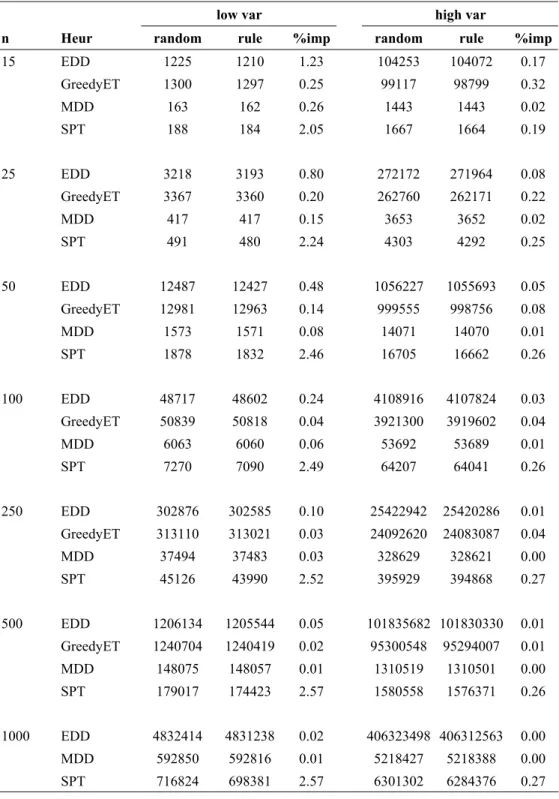
In Table 1, we present the average objective function value for both the heuristic versions that break the ties randomly (random), and the versions that use problem-related criteria (rule). We also give the relative improvement in the average objective function value
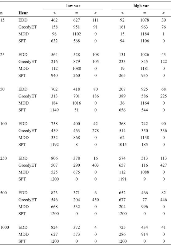
(%imp), calculated as (random – rule) / random × 100. In Table 2, we give the number of
instances for which the versions with a tie breaking rule performed better (<), equal (=) or worse (>) than the versions with a random tie break. We also performed a test to determine if the difference between the two versions is statistically significant. Given that the two versions were used on exactly the same problems, a paired-samples test is appropriate. Since some of the hypotheses of the paired-samples t-test were not met, the non-parametric Wilcoxon test was selected. The significance values of this test, i.e., the confidence level values above which the equal distribution hypothesis is to be rejected, were always equal to 0.000. From the results presented in these two tables, we can conclude the following. The versions that use a problem-related tie breaking criterion outperform the random versions, since their average objective function value is lower and they provide better results for a (sometimes quite) large number of the test instances. The Wilcoxon test values also indicate that the difference in distribution between the two versions is statistically significant.
Table 1 – Objective function value and relative improvement.
low var high var
n Heur random rule %imp random rule %imp
15 EDD 1225 1210 1.23 104253 104072 0.17
GreedyET 1300 1297 0.25 99117 98799 0.32
MDD 163 162 0.26 1443 1443 0.02
SPT 188 184 2.05 1667 1664 0.19
25 EDD 3218 3193 0.80 272172 271964 0.08
GreedyET 3367 3360 0.20 262760 262171 0.22
MDD 417 417 0.15 3653 3652 0.02
SPT 491 480 2.24 4303 4292 0.25
50 EDD 12487 12427 0.48 1056227 1055693 0.05
GreedyET 12981 12963 0.14 999555 998756 0.08
MDD 1573 1571 0.08 14071 14070 0.01
SPT 1878 1832 2.46 16705 16662 0.26
100 EDD 48717 48602 0.24 4108916 4107824 0.03
GreedyET 50839 50818 0.04 3921300 3919602 0.04
MDD 6063 6060 0.06 53692 53689 0.01
SPT 7270 7090 2.49 64207 64041 0.26
250 EDD 302876 302585 0.10 25422942 25420286 0.01
GreedyET 313110 313021 0.03 24092620 24083087 0.04
MDD 37494 37483 0.03 328629 328621 0.00
SPT 45126 43990 2.52 395929 394868 0.27
500 EDD 1206134 1205544 0.05 101835682 101830330 0.01
GreedyET 1240704 1240419 0.02 95300548 95294007 0.01
MDD 148075 148057 0.01 1310519 1310501 0.00
SPT 179017 174423 2.57 1580558 1576371 0.26
1000 EDD 4832414 4831238 0.02 406323498 406312563 0.00
MDD 592850 592816 0.01 5218427 5218388 0.00
Table 2 – Objective function value comparison.
low var high var
n Heur < = > < = >
15 EDD 462 627 111 92 1078 30
GreedyET 158 951 91 161 963 76
MDD 98 1102 0 15 1184 1
SPT 632 568 0 94 1106 0
25 EDD 564 528 108 131 1026 43
GreedyET 216 879 105 233 845 122
MDD 112 1088 0 19 1181 0
SPT 940 260 0 265 935 0
50 EDD 702 418 80 207 925 68
GreedyET 313 701 186 389 586 225
MDD 184 1016 0 36 1164 0
SPT 1149 51 0 656 544 0
100 EDD 758 400 42 368 742 90
GreedyET 459 463 278 514 350 336
MDD 332 868 0 62 1138 0
SPT 1192 8 0 1015 185 0
250 EDD 806 378 16 574 513 113
GreedyET 507 290 403 657 116 427
MDD 525 675 0 112 1088 0
SPT 1200 0 0 1191 9 0
500 EDD 823 371 6 652 466 82
GreedyET 546 204 450 677 77 446
MDD 668 532 0 204 996 0
SPT 1200 0 0 1200 0 0
1000 EDD 824 372 4 725 434 41
MDD 627 573 0 286 914 0
The number of instances for which the rule-based versions give better results increases with the instance size. However, the relative improvement decreases as n increases for the MDD, EDD and GreedyET heuristics, while it tends to increase for the SPT dispatch rule. This latter result concerning the SPT rule is not surprising. In fact, as the instance size increases, the number of jobs sharing the same processing time also increases. Therefore, more ties will take place, and the extra information given by the problem-related criterion is used a larger number of times. The variability of the processing times and penalties does not seem to have much effect on the GreedyET heuristic, though it significantly affects the other procedures. For the MDD, SPT and EDD heuristics, both the relative improvement and the number of instances for which a better result is obtained are much higher when the variability is low. This effect of the processing times and penalties variability is to be expected. When the variability of the processing times is low, more jobs share the same pj, and therefore more
ties will occur in the SPT dispatch rule. Also, when the processing time variability is low, the intervals in which the due dates are contained are tighter, since P, the sum of the pjs, is smaller. The probability of two jobs having identical due dates is then higher, and more ties will take place in the EDD heuristic. The number of ties will also be larger in the MDD heuristic when the probability of two jobs having identical due dates and processing times is higher.
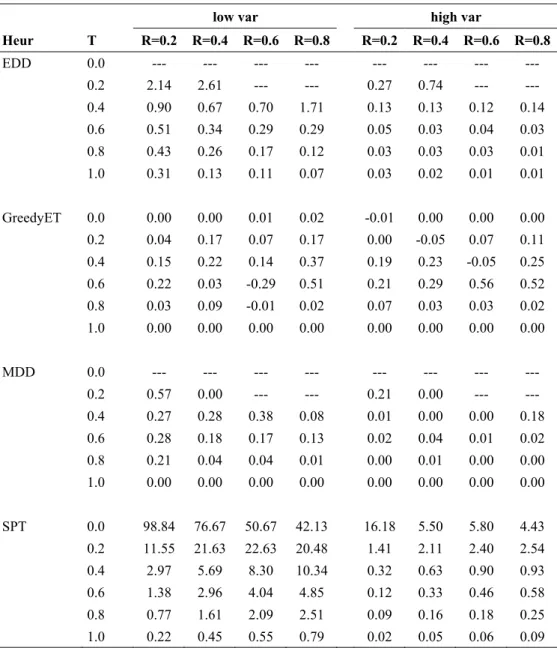
The effect of the T and R parameters on the relative objective function value improvement is given in Table 3 for instances with 100 jobs. From the results presented in this table, we can see that the tardiness factor T has a significant effect on the relative improvement provided by the rule-based tie break criterion. In the case of the GreedyET heuristic, the relative improvement is higher for instances with a tardiness factor of 0.4 or 0.6. The improvement decreases as T approaches its extreme values, and is mostly inexistent when T is equal to 0.0 or 1.0. This result is to be expected, since the early/tardy problem is more difficult for the intermediate T values. If all jobs are necessarily early (late), an optimal schedule can easily
be obtained, and when T = 0.0 (1.0), most jobs will indeed be early (late). For the
intermediate T values, there is a greater balance between the number of early and tardy jobs, and the problem becomes more difficult. Therefore, there are more possibilities for improvement when T is equal to 0.4 or 0.6 (i.e., when the problem is harder).
For the MDD, SPT and EDD heuristics, the relative improvement is lower when T = 1.0, and
then gradually increases as T decreases towards 0.2. For some parameter combinations,
namely for T = 0.0, or when T = 0.2 and R is equal to 0.6 or 0.8, the optimal solution for most or all instances of the weighted and unweighted tardiness problems has no tardy jobs, and therefore the optimal objective function value is zero. The --- sign in the MDD and EDD results corresponding to these parameter values means that both versions of these heuristics obtained such an optimal solution for all instances with these parameter combinations. The relative improvement values of the SPT heuristic are also quite high for these same parameter combinations. These values are somewhat misleading, since they correspond to situations where the average objective function value is quite low for both versions. The decrease in the total tardiness made possible by the rule-based criterion is therefore small
when measured in absolute terms. When T = 1.0, most jobs will be tardy, and both the
weighted and unweighted tardiness problems are easy to solve. As T decreases, the
Table 3 – Relative improvement for instances with 100 jobs.
low var high var
Heur T R=0.2 R=0.4 R=0.6 R=0.8 R=0.2 R=0.4 R=0.6 R=0.8
EDD 0.0 --- --- --- --- --- --- --- ---
0.2 2.14 2.61 --- --- 0.27 0.74 --- ---
0.4 0.90 0.67 0.70 1.71 0.13 0.13 0.12 0.14
0.6 0.51 0.34 0.29 0.29 0.05 0.03 0.04 0.03
0.8 0.43 0.26 0.17 0.12 0.03 0.03 0.03 0.01
1.0 0.31 0.13 0.11 0.07 0.03 0.02 0.01 0.01
GreedyET 0.0 0.00 0.00 0.01 0.02 -0.01 0.00 0.00 0.00
0.2 0.04 0.17 0.07 0.17 0.00 -0.05 0.07 0.11
0.4 0.15 0.22 0.14 0.37 0.19 0.23 -0.05 0.25
0.6 0.22 0.03 -0.29 0.51 0.21 0.29 0.56 0.52
0.8 0.03 0.09 -0.01 0.02 0.07 0.03 0.03 0.02
1.0 0.00 0.00 0.00 0.00 0.00 0.00 0.00 0.00
MDD 0.0 --- --- --- --- --- --- --- ---
0.2 0.57 0.00 --- --- 0.21 0.00 --- ---
0.4 0.27 0.28 0.38 0.08 0.01 0.00 0.00 0.18
0.6 0.28 0.18 0.17 0.13 0.02 0.04 0.01 0.02
0.8 0.21 0.04 0.04 0.01 0.00 0.01 0.00 0.00
1.0 0.00 0.00 0.00 0.00 0.00 0.00 0.00 0.00
SPT 0.0 98.84 76.67 50.67 42.13 16.18 5.50 5.80 4.43
0.2 11.55 21.63 22.63 20.48 1.41 2.11 2.40 2.54
0.4 2.97 5.69 8.30 10.34 0.32 0.63 0.90 0.93
0.6 1.38 2.96 4.04 4.85 0.12 0.33 0.46 0.58
0.8 0.77 1.61 2.09 2.51 0.09 0.16 0.18 0.25
1.0 0.22 0.45 0.55 0.79 0.02 0.05 0.06 0.09
4. Conclusion
In this paper, we analysed the effect of using appropriate tie breaking criteria in dispatch rules for scheduling problems. Four different dispatch procedures were considered, and for each of these heuristics we compared two versions that differ only in the way ties are broken. The first version breaks ties randomly, while the second uses a criterion that incorporates problem-specific knowledge.
The computational results show that using adequate tie breaking criteria improves the performance of the dispatch heuristics, with virtually no additional computational effort. The magnitude of the improvement, however, was quite different for the four heuristics. The improvement also depends on the characteristics of each specific instance. As expected, the improvement is more significant for instances where the probability of occurring ties is higher. The effectiveness of the problem-based tie breaking criteria is also greater for the more difficult instances, where there are more possibilities for improvement. The use of problem-related knowledge for breaking ties should therefore be given some consideration in the implementation of dispatch rules, particularly when they are used in production scheduling systems.
Acknowledgement
The author would like to thank the anonymous referees for several helpful comments and suggestions that were used to improve this paper.
References
(1) Baker, K. R. & Bertrand, J. W. M. (1982). A dynamic priority rule for scheduling
against due dates. Journal of Operations Management, 3, 37-42.
(2) Fadlalla, A.; Evans, J. R. & Levy, M. S. (1994). A greedy heuristic for the mean
tardiness sequencing problem. Computers & Operations Research, 21, 329-336.
(3) Jackson, J. R. (1955). Scheduling a production line to minimize maximum tardiness.
Management Science Research Project, Research Report 43, University of California, Los Angeles.
(4) Morton, T. E. & Pentico, D. (1993). Heuristic Scheduling Systems. Wiley,
New York.
(5) Ow, P. S. & Morton, E. T. (1989). The single machine early/tardy problem.
Management Science, 35, 177-191.
(6) Pinedo, M. (1995). Scheduling: Theory, Algorithms and Systems. Prentice Hall,
New Jersey.
(7) Pinedo, M. & Chao, X. (1999). Operations Scheduling with Applications in
Manufacturing and Services. McGraw-Hill, Singapore.
(8) Smith, W. E. (1956). Various optimizers for single-stage production. Naval Research
(9) Valente, J. M. S. & Alves, R. A. F. S. (2005). Improved heuristics for the early/ tardy scheduling problem with no idle time. Computers & Operations Research, 32, 557-569.