Flow Induced Vibration, Zolotarev & Horacek eds. Institute of Thermomechanics, Prague, 2008 FLOW-ACOUSTIC INTERACTION IN CORRUGATED PIPES:
TIME-DOMAIN SIMULATION OF EXPERIMENTAL PHENOMENA
V. Debut & J. Antunes
Institute of Nuclear Technology, Applied Dynamic Laboratory, Sacav´em, Portugal
M. Moreira
Polytechnic Institute of Setubal, Department of Mathematics, Setubal, Portugal
ABSTRACT
A phenomenological model based on the coupling between a set of “pressure vortex oscillators” and an acoustic field is considered to simulate the dynamical behaviour of a corrugated pipe. The effect of a random Gaussian dispersion of the Strouhal number is investigated by means of non-linear numerical time-domain simulations and also in terms of the modeshapes of the linearized aeroacoustical model. The results demonstrate that such perturbations may qualitatively change the dynamics of the model and might cause local-ization phenomenon.
1. INTRODUCTION
In the context of aerodynamic noise generation, a corrugated pipe open at both ends emits clear and loud tones when air flows through it at suf-ficiently high velocities. This tone generation - also called whistling - is an example of flow-excited acoustic phenomenon, in which air-flow interacts with the longitudinal acoustic modes of the duct to give rise to self-sustained oscilla-tions. Due to its pratical significance in a large variety of technical applications and its intricate fundamental aspects, the phenomenon is being currently studied by different authors by means of experiments (Belfroid et al. (2007); Kristiansen and Wiik (2007)) as well as numerical simula-tions (Popescu and Johansen (2008)). To main-tain the acoustic oscillations, the central physi-cal feature is a lock-in phenomenon between the resonant acoustic field in the pipe and a vortex shedding process due to the passage of air-flow over the corrugations. The aeroacoustic insta-bility occurs when the frequency of the vortex shedding, characterized by a Strouhal number
St, approaches the frequency of one of the nat-ural acoustic modes of the pipe. The whistling frequencies are the natural harmonics stemming from the tube acoustical modes, and the modes
which actually become unstable depend on the air-flow velocity, the tube length and corrugation geometry.
In a recent paper (Debut et al. (2007a)), the authors reported preliminary experiments for a number of corrugated pipes with different diam-eters, length and corrugation lengths. They con-firmed most of the qualitative behaviour reported in the literature (Petrie and Huntley (1980); Nakamura and Fukamachi (1991)) and showed that many features observed are not easy to ex-plain. No simple scaling relation was found to characterize the physical phenomenon: the oper-ating Strouhal number based on the corrugation pitch is in the range 0.4∼0.5 for all tested tubes. Moreover, it was observed that the condition for a self-sustained regime to arise concerning the co-incidence of the vortex shedding frequency with the frequency of one of the pipe acoustic modes is necessary but not sufficient.
presented to illustrate how the model behaves. Because the underlying physics may evolve in an irregular fashion due the rather ill-defined sepa-ration point of the vortices, the irregular corru-gation geometry and pitch, as well as the pres-ence of highly turbulent pipe flow, it is of in-terest to consider the case of a random Gaus-sian dispersion on the Strouhal number. Non-linear numerical simulations highlight the quali-tative changes in the dynamical behaviour. Fi-nally, considering the linearized coupled formula-tion, the phenomenon of localization of the nor-mal mode shape is discussed.
2. THE COUPLED NONLINEAR MODEL
2.1. Acoustic pressure field
The acoustic pressure p(x, t) at location x for the case when an external force field fx(x, t) is
considered, is solution of the inhomogenous wave equation given by
1
c2
∂2
p
∂t2 −
∂2
p
∂x2 =−
∂fx
∂x (1)
wherecis the sound speed. Considering a line of
N discrete “equivalent” pressure source Pn
dis-tributed along the pipe at N locationsxn, Eq.(1)
becomes
∂2
p
∂t2 −c
2 ∂ 2
p
∂x2 =−c
2 N
X
n=1
Pnδ′(x−xn) (2)
where δ′(x−xn) is the spatial derivative of the Dirac function evaluated at locationx=xn.
2.2. “Pressure vortex oscillator” dynam-ics
The shedding of vortices stemming from a corru-gation located at each x =xn is here described
phenomenologically by a non-linear Van der Pol equation given by
¨ Pn+A
"
Pn
B Vα
2
−1
#
ωsP˙n+ω
2
sPn=Cp′(xn, t)
(3) and referred to as “pressure vortex oscillator”. Parameter A controls the strengh of the non-linear damping and parameter B is related to the size of the stable limit cycle which is assumed to vary with the flow velocity as Vα. ω
s is the
Strouhal frequency. The right-hand side forcing term models the effect of the pressure field on the
oscillator at the oscillator location. Note that the pressure field acts via its spatial derivative
p′(x
n, t) = [∂p(x, t)/∂x]x=xn proportionnaly to
the coupling parameter C. Such coupling is in accordance with Howes analogy, where acoustic energy generation involves the acoustic velocity in the source region (Hirschberg (1995)).
2.3. Computational modal formulation
To solve the coupled problem formed by Eqs. (2) and (3), we use a modal approach in which the pressure field is expanded as the modal series:
p(x, t) =
M
X
m=0
qm(t)Φm(x) (4)
where qm(t) are the modal amplitudes and
Φm(x) = sin(mπx/L) are the pressure
mode-shapes for a pipe of length L with both ends opened (m ∈ N). Replacing the modal expan-sion of the pressure field in Eqs.(2) and (3), mul-tiplying by a modeshape Φq, integrating within
the domain [0, L] and accounting for the modal orthogonality relation, RLΦm(x)Φq(x)dx= L/2
for m=p=1,2,. . . , we finally obtain the set of (N+M) modal ODEs
¨
qm+ 2ζmωmq˙m+ω2mqm =
2c2 L
N
X
n=1
Pn(t)Φ′m(xn)
¨ Pn+A
"
Pn
BVα
2
−1
#
ωsP˙n+ωs2Pn=
=C M
X
m=1
qm(t)Φ′m(xn)
(5)
To investigate the dynamics of the coupled non-linear model (5), time-domain numerical com-putations are performed using a time-step inte-gration algorithm presented in (Hart and Wong (1999)). Time histories and spectra of both the pressure field and source variables are com-puted and evaluation of the instantaneous fre-quency and amplitude of the dominant mode is done using the Hilbert transform (Oppenheim and Schafer (1998)).
3. LINEARIZED MODAL
FORMULATION FOR THE COUPLED MODEL
with a bar the mean quantitites and with a hat oscillating quantities, pressure and vortex oscil-lators displacement quantities are written as
p(x, t) =p(x) + ˆp(x, t) (6)
Pn(x, t) =Pn(x) +Pnc(x, t) (7)
The subsitution of (6) and (7) into Eqs.(2) and (3) leads to two sets of equations: the zero-order equations which govern the steady state solu-tions, and the first-order equations which gov-ern the oscillating solutions of the coupled prob-lem. To apply the modal projection method to the obtained equations, both the steady and the oscillating pressure field are expanded as modal series:
p(x) =
M
X
m=0
qmΦm(x), pˆ(x, t) =
M
X
m=0
ˆ
qm(t)Φm(x)
(8) The first-order equations are in the form of:
¨ ˆ
qm+ 2ζmωmq˙ˆm+ω
2 mqˆm =
2c2 L
N
X
n=1
c
Pn(t)Φ′m(xn)
¨
c
Pn−AωsPc˙n+ωs2Pcn=C M
X
m=1
ˆ
qm(t)Φ′m(xn)
(9) Complex eigenvalues and eigenvectors of the lin-earized formulation are obtained by assuming harmonic solutions to the first-order equations (9) in the usual manner (see Pierce (1981)).
4. BASIC SIMULATIONS
For the presented simulations, the pipe length was set to L=1 m and a modal damping of 0.5% was assumed for all acoustical modes. The self-excited oscillators were uniformely spaced along the pipe. Initial conditions for the vortex os-cillators were taken as small random amplitudes of the variables of order 10−4
, all the acoustical variables being zero. N=101 “vortex oscillators” and M=10 modes are considered. A reference Strouhal numberSt=0.4 is assumed.
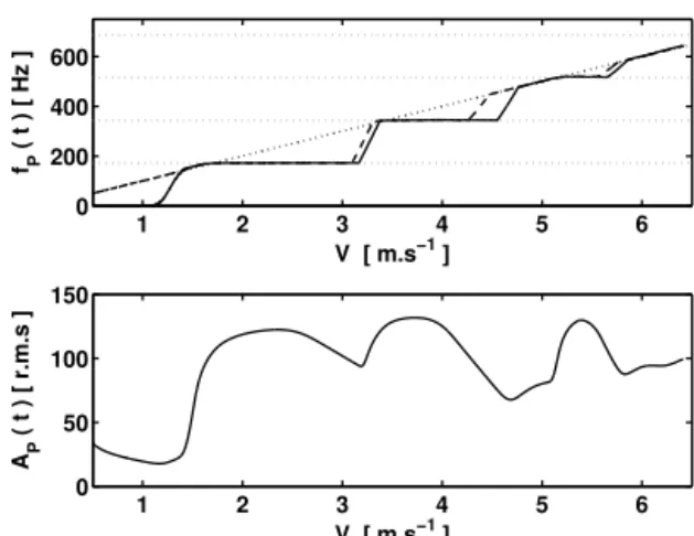
Figure 1 illustrates the case of strong coupling for which the phenomenon of frequency lock-in is clearly observed. The following parameters are used: A=0.005, B=0.0001, C=-200 and α=3. It represents the instantaneous frequencies for the acoustic pressure and oscillators variables when a linear sweep is imposed on the “vortex oscillator” characteristic frequency by means of an increas-ing flow velocity. Several qualitative observations
1 2 3 4 5 6
0 200 400 600
V [ m.s−1 ]
fP
( t ) [ Hz ]
1 2 3 4 5 6
0 50 100 150
V [ m.s−1 ]
AP
( t ) [ r.m.s ]
Figure 1: Increasing linear velocity sweep on the characteristic frequency of the vortex oscillators for a perfectly tuned 101-oscillator pipe. Case for strong coupling. A=0.005, B=0.0001,
C=-200, α=3. Instantaneous frequency and
ampli-tude of the internal pressure at the oscillator lo-cation x10=0.0982 m. The frequency of the os-cillator has been superposed with dashed line (--) to highlight the lock-in stages. The dots in the diagonal represents the Strouhal law. Horizontal dots are for the pipe modal frequencies.
1 2 3 4 5 6
0 200 400 600
V [ m.s−1 ]
fP
( t ) [ Hz ]
1 2 3 4 5 6
0 50 100 150
V [ m.s−1 ]
AP
( t ) [ r.m.s ]
assert the presence of frequency lock-in: first, the entrainment of the “pressure vortex oscillators” by the pressure field; then, the mutual adjust-ment of the frequencies in a given range of flow velocities; finally, the presence of large pressure pulsations in these regions. Moreover, by com-parison with the plot in Figure 2 where the case ofweak coupling is considered, one observes that the strength and the extent of lock-in are strongly controlled by the coupling parameter C.
5. DISPERSION ON THE VORTEX STROUHAL NUMBER
Departure from regularity in the geometrical con-figuration might be expected in corrugated pipes. In such spatially extended periodic structures, disorder might strongly influence the vortex gen-eration, as well as the propagation of waves, by causing the phenomenon of localization (Hodges (1981)). Here, we allow some disorder in the sys-tem by assuming that the vortex shedding pro-cess differs slightly for each corrugation. Disor-der is simulated as a random variation of the Strouhal number defined with a Gaussian dis-tribution. Looking at Eqs.(5), we are now con-cerned with an ensemble of self-excited oscillators with slightly different characteristic frequencies interacting via the acoustic field. The question of self-organization of the model to evolve coher-ently with the same frequency has to be recon-sidered. Intuitively, it may be that at least some oscillators lock on a common frequency (and thus contribute to the pressure field) whereas others are nonentrained and oscillate at their own fre-quency. Thus, the onset of a collective lock-in, if possible, may be less predictable than for the tuned case - depending on the distribution of the Strouhal frequencies, the oscillator locations and the coupling strength. In the next section, we provide a first examination of the effect of dis-order in the nonlinear model (5) by means of numerical simulations. Finally, we examine the occurence of localization in terms of the normal modeshapes of the coupled linearized formulation (9).
5.1. Time domain simulations
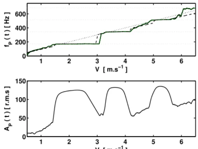
From the nonlinear dynamical point of view, we present results of numerical simulations in Fig-ures 3 and 4 when considering a random pertur-bation with a standard deviationσ= 0.02 added to the reference Strouhal number St=0.4. In comparison with the plot at Figure 1, Figure 3
1 2 3 4 5 6
0 200 400 600
V [ m.s−1 ]
fP
( t ) [ Hz ]
1 2 3 4 5 6
0 50 100 150
V [ m.s−1 ]
AP
( t ) [ r.m.s ]
Figure 3: Increasing linear velocity sweep on the characteristic frequency of the vortex oscillators for a mistuned 101-oscillator pipe. Strong cou-pling C=-200. Standard deviation of St,σ=0.02. Same legend as in Figure 1.
2 4 6 8
0 500 1000
V [ m.s−1 ]
f P
( t ) [ Hz ]
2 4 6 8
20 40 60 80 100
V [ m.s−1 ]
AP
( t ) [ r.m.s ]
Figure 4: Increasing linear velocity sweep on the characteristic frequency of the vortex oscillators for a mistuned 101-oscillator pipe. Weak cou-pling C=-30. Standard deviation of St, σ=0.02. Same legend as in Figure 1.
4.5 5 5.5 6
400 500 600
V [ m.s−1 ]
fP
( t ) [ Hz ]
4.5 5 5.5 6
50 100 150
V [ m.s−1 ]
AP
( t ) [ r.m.s ]
Figure 5: Increasing linear velocity sweep on the characteristic frequency of the vortex oscil-lators for a mistuned 101-oscillator pipe around the frequency of the third acoustic pipe mode. Strong coupling C=-200. Standard deviation of
clearly shows some quantitative changes. Partic-ularly, some lock-in ranges are shortened and the threshold velocities defining the stable/unstable character of each acoustic mode are altered. It is observed that the velocity ranges for which an acoustic mode is unstable are broadened (see Fig-ure 5) and that the transitions between modal jumps are less marked. An important decrease in the amplitude of the acoustic pressure is also observed between two successive stages although amplitude maxima remains large within lock-in. Figure 4 is obtained for the case ofweakcoupling with a standard deviationσ=0.02.
Contrary to the case with identical Strouhal number oscillators, computed time-history sig-nals are not always stationnary. Strickly speak-ing, the frequencies of the “vortex oscillators”
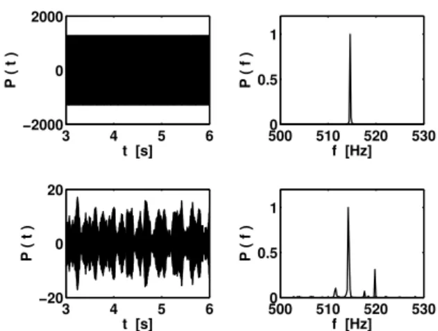
nearly adjust with the pipe natural frequencies. In addition, several oscillators might have uncor-related movement during an aeroacoustic insta-bility and thus the all-to-all complete time-space correlation between the “vortex oscillators” does not appear necessary to explain the excitation of the acoustic field. Indeed, it is quite reasonable to state that lock-in still exists, because the ratio of the instantaneous frequencies of the interact-ing oscillators and pressure field remains approx-imatively constant in a range of flow velocities. These remarks are illustrated in Figure 4. Figure 6 shows the time envelopes and corre-sponding spectra for tuned and mistuned cases under constant excitation. Looking at the spec-trum for the mistuned case, one notices the pres-ence of closely located distinct peaks distributed in a narrow band region about a central fre-quency, as reported in (Elliot (2005); Debut et al. (2007a)). In the time-domain, the correspond-ing amplitude modulation effect is observed and can be clearly heard from the corresponding com-puted sound. This suggests that modeling ran-dom phenomena may be of importance. Looking at the pressure amplitude, note the strong atten-uation for the mistuned case. It has also been ob-served that the entrainment of the oscillators may be prevented for large mistuning (σ ∽0.1) caus-ing a strong attenuation for the acoustic pressure field. As a result, mistuning appears as a stabiliz-ing factor for the coupled system. This observa-tion is supported by the qualitative remarks pro-vided by Petrie and Huntley (Petrie and Huntley (1980)) who noticed that very small differences in corrugation shape eliminate the whistle.
3 4 5 6
−2000 0 2000
t [s]
P ( t )
5000 510 520 530
0.5 1
f [Hz]
P ( f )
3 4 5 6
−20 0 20
t [s]
P ( t )
5000 510 520 530
0.5 1
f [Hz]
P ( f )
Figure 6: Time envelopes and corresponding nor-malized autospectrum for a constant excitation of the third mode (fs = f3). Tuned (up) and mistuned (down) cases for a 101-oscillator pipe. Strong coupling C=-200. Standard deviation of
St, σ=0.02.
5.2. Effect on the modeshapes
The linearized modal equations for the coupled problem (9) enable to study the system stability through the computation of its complex eigenval-ues and eigenvectors. As illustrated on Figure 7 for the first mode of a perfectly tuned 101-vortex oscillators pipe during lock-in, a global coher-ent vibration of the vortex oscillators can easily synchronize with the acoustic modes specifically with the space derivative of the pressure field (see Eq.(3)). As the degree of mistuning increases, its effect is clearly seen on the vortex oscillators re-sponses, localizing their action in a small region of the pipe. For the corresponding unstable mode of the coupled system, we observe that the neg-ative modal damping decreases as the standard deviationσ increases. Notice also the slight dis-torsion for the pressure coupled modeshape as the mistuning becomes stronger.
6. CONCLUSIONS
Based on a phenomenological model dealing with the aeroacoustic coupling between a line of “pres-sure vortex oscillators” with an acoustic field, numerical time-domain simulations for a corru-gated pipe were performed. It was found that including random perturbation on the Strouhal number might qualitatively change the dynam-ical behaviour of the nonlinear model. Under certain circumstances, the threshold values for the instability of an acoustical mode are altered and the model succeeds in simulating the “noisy” sound observed experimentally for high flow ve-locities. Considering the linearized formulation for the coupled system, localization has been ob-served, the acoustical modeshapes being then slightly distorded in comparison with those for the unperturbed case. However, it is important to note that all our observations clearly depend on the relative strength between the random per-turbations and the coupling parameter magni-tude. It is interesting to note that, in Figure 4, the qualitative evolution of the amplitude is quite well reproduced compared to experiments. Finally, because of the high level of turbulence in the pipe flow and in the light of these results, it will be interesting to include a model for the turbulence disturbance acting on the “vortex os-cillators”.
7. ACKNOWLEDGEMENTS
This work was supported financially by the Por-tuguese Fondation of Sciences and Technology (project number POCTI/EME/57278/2004).
8. REFERENCES
Belfroid S.P.C., Peters R.M.C.M. and Shatto D.P, 2007, Flow induced pulsations caused by corrugated tubes”. ASME Pressure Vessels and Piping Division Conference, San Antonio. Debut V., Antunes J., Moreira M., 2007, Ex-perimental Study of the Flow-Excited Acousti-cal lock-in in a Corrugated Pipe. In 14thICSV Proceedings, Cairns.
Debut V., Antunes J., Moreira, M., 2007, Phe-nomenological model for sound generation in corrugated pipes. In ISMA2007 Proceedings, Barcelona.
Elliot J. W., 2005, Lectures Notes on the Math-ematics of Acoustics. Imperial College Press. Facchinetti M., De Langre E., Biolley F., 2003, Coupling of structure and wake oscillators in vortex-induced vibrations. In J.of Fluids and Structures.
Hart G. C., Wong K., 1999, Structural Dynamics for Structural Engineers. p.58-60. Wiley.
Hirschberg A., 1995, Aero-acoustics of wind in-struments. InMechanics of musical instruments, CISM Courses and Lectures. Springer-Verlag. Hodges H.C., 1981, Confinement of vibration by structural irregularity. In J. Sound and Vib., 82:411-424.
Kristiansen Ulf. R., Wiik Geir A., 2007, Exper-iments on sound generation in corrugated pipes with flow. InJ.Acoust.Soc.Am.,121:1337-1344. De Langre, E., 2006, Frequency lock-in is caused by coupled-mode flutter. In J.Sound and Vib., 265: 359-386.
Nakamura Y., Fukamachi N., 1991, Sound gen-eration in corrugated tubes. In Fluids Dynamics Research,7:255-261.
Oppenheim A.V., Schafer R.W., 1998, Discrete-Time Signal Processing. Prentice Hall.
Petrie A. M., Huntley I. D., 1980, The acoustic output produced by a steady airflow through a corrugated duct. InJ.Sound and Vib.,70:1-9. Pierce Allan D., 1981, Acoustics, an introduc-tion to its physical principles and applicaintroduc-tions. McGraw-Hill.