DOI: 10.14636/1734-039X_11_1_004
We investigate several promising algorithms, proposed in literature, devised to detect sudden changes (structural breaks) in the volatility of financial time series. Comparative study of three techniques: IC““, NPCPM a d Che g’s algo ith is carried out via numerical simulation in the case of simulated T-GARCH models and two real series, namely German and US stock indices. Simulations show that the NPCPM algorithm is superior to ICSS because is not over-sensitive either to heavy tails of market returns or to their serial dependence. Some signals generated by ICSS are falsely classified as structural breaks in
olatility, hile Che g’s tech i ue o ks ell o ly he a single break occurs.
JEL classification: C19, C22, C58.
Keywords: volatility, structural breaks, financial time series, logarithmic returns, Threshold-GARCH model
Received: 30.09.2014 Accepted: 18.05.2015
Acknowledgement
This paper is supported by scientific grant No. UMO-2013/10/M/ST1/00096, financed by NCN, Poland, within
Ha o ia 5 esea ch p og a e.
1
33
Volatility is one of the all-important terms in financial econometrics, where dynamics of asset price processes, currency valuations and various economic data are the subject of research. Even though its multiple quantitative definitions are proposed, volatility can be viewed as a measure of the unpredictability of a given time series’ (like asset returns) behavior within an analyzed time span. It has been an object of intensive research for several decades now, as its proper understanding and description provides a cutting edge in trading on stock exchanges, portfolio and risk management, stress testing, etc. Formally, financial volatility can be a parameter (either constant or another stochastic process itself) present in the model driving the given price dynamics, eg. σ in Geometric Brownian Motion. The crucial role of this parameter in derivatives pricing emerges in the celebrated Black-Scholes option pricing formula dating back to 1973. Whenever computation and modelling is involved, volatility is estimated by a sample standard deviation of logreturns, but interpreting it as unconditional variance is also commonplace among practitioners.
One of the empirically and widely stated hindrances, however, is that in many practical applications volatility evolves over time. It may have its separate stochastic dynamics proposed, leading to the concept of stochastic volatility models. Another approach, adequate in numerous cases, allows for sudden changes (structural breaks) occurring at the moment when some external shocks or other unexpected, profound shifts in economic background happen. A vast class of so-called threshold models has been proposed to handle these peculiarities more effectively. Here, rather than on price dynamics modelling issues, we will focus on the problem of detection of structural breaks in volatility, employing several promising techniques proposed in the literature cited successively below. (Mean or median change point estimation, albeit also prominent in research, is not addressed here.) Worth mentioning, irrespective of the solely econometric background we will stick to hereafter, is that the problem of volatility break detection is relevant also in other scientific areas such as climatology, medical sciences or mechanics.
The paper is organized as follows. In Section 2 we formally set up the problem and after a brief discussion and references summary, we cite with more detail three known techniques of structural break detection, providing basic source theorems justifying their applicability. Section 3, being fundamental, presents comparison of these algorithms applied for simulated (with intended breaks at some time points) and real financial time series. Detailed computational results for simulated Threshold-GARCH models and two real indice quotes data are provided therein. We numerically show the irrelevance of the Cheng algorithm (discussed below) in the case of multiple volatility breaks. Section 4 contains conclusions and discussion of vital problems concerning stochastic modeling with presence of structural breaks. Finally, literature references are provided.
Let {St}t=0,…,T be a discretely observed asset price process, eg. daily record of an equity or stock index quotes.
Logarithmic returns, in short logreturns are defined as:
/
1
log
t tt
S
S
R
,
t
=1,…,
T
. (1)
In the pioneer econometric literature, it was assumed that {Rt}t=,…,T ~ iid N(0,σ
2
34
logreturns leptokurticity the stringent normality assumption was gradually relaxed. Further ample research showed that iid case in most situations was still too rigorous, paving the way eg. for conditionally heteroscedastic GARCH models proposed by Bollerslev (1986). However, all these cases (GARCH being weakly stationary) are characterized by constant unconditional variance σ2, which translates into constant volatility within the discussed time span. Such an assumption may lead to the choice of a wrongly specified model for dynamics of {Rt}, amplifying the risk of erroneous statistical inference, poor forecasting performance, etc.
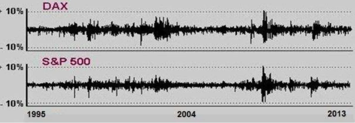
Doubts as to whether unconditional volatility is indeed flat over time may arise just upon a brief graphical inspection of asset return series over a sufficiently long time horizon. Alternate periods of lower and higher volatility, the phenomenon called clustering, is clearly evident in Figure 1, which presents daily logreturns series of (German) DAX30 and (USA) S&P500 indices throughout nearly 19 years, until November 2013. The 2008 crash is especially strongly pronounced.
Figure 1: Logreturns of DAX30 and S&P500 stock indices; Jan 2, 1995 – Nov 7, 2013
Source: Autho ’s own computations and graph based on data provided by www.bossa.pl
Such behavior can be captured to some extent by GARCH series, but the optimal model fitted is quite often close to a stationarity boundary, which in turn diminishes its applicational value. Another but more sophisticated tool for examining the volatility evolution is provided by the Chicago Board of Options Exchange, which since 2004 has been offering a synthetic volatility index (VIX) as a quotable and tradable asset. Without going into technical details insubstantial for our purposes, we only mention that it is computed as an annualized, implied volatility averaged-out from at-the-money call and put S&P500 options with ca. monthly maturity, measured in vol points. Full description of the asset can be found on www.cboe.com. Figure 2 shows its 9-year trajectory.
Figure 2: Nine-year series of VIX index quotes through Nov. 7, 2013
Source: Autho ’s own graph based on data acquired from www.cboe.com
35
smoothly give up as the market dynamics reverse to the complacent mode indicated by sub-20 vol points levels. From our perspective it seems therefore promising to detect these breaks by employing targeted algorithms, some of which are in their nature statistical tests.
Within the series {Rt}t= ,…,T we want to detect a possible single or multiple volatility break. More precisely, we aim at possibly the most accurate identification of the moments the changes occur, namely 1 < τ1<…< τK < T; K << T. Under these breaks, the unconditional variance evolves over time in a piecewise constant manner:
t2
2j for
j1
t
j,1
j
K
1
, where for convenience we define starting and ending valuesT
K
10
1
,
.Until now, under one or multiple volatility break(s) setup quite a few approaches have been proposed, resulting in concurrent detection algorithms. In the pioneer paper of Inclán and Tiao (1994), henceforward I&T, a CUSUM-type test for detecting a variance structural break in the iid Gaussian case was derived. The procedure was then carried out iteratively to handle multiple breaks, thus providing an ICSS algorithm being the subject of Section 2.1. More extensive empirical application of this procedure for financial time series can be found in Aggarwal et al. (1999). However, the ICSS method employed in econometrics faced justified iti is y “a só, Arago and Carrion-i-Silvestre (2004), as its fundamental assumptions are not met. Data are neither Gaussian, nor iid, causing poor performance of this tool. Indeed, many spurious (false) change points may be flagged due to
fat-tailed distribution of Rt’s (generating outliers) instead of a real structural volatility break. Moreover, serial dependence and conditional heteroscedasticity pose separate sources of test size distortions. A o di gly, “a só et al. (2004) robustified the original ICSS method to handle leptokurticity and lack of independence, including GARCH effects. Kokoszka and Leipus (2000) provided a CUSUM-type consistent estimator of a single break point within a possibly non-Gaussian ARCH() framework. Cheng (2009) proposed a more efficient and numerically economical algorithm for change-point detection, encompassing among others the volatility break case. This technique is explained closer in Section 2.2 below. Alternatively, a more recent paper of Ross (2013) presented a nonparametric approach, based on the lassi Mood’s a k test dating back to 1954. The old tool was applied to specific financial time series, and its iterative version for multiple break detection was performed, yielding a non-parametric change-point algorithm (NPCPM). We focus on this procedure in Section 2.3. Xu (2013) presented a nonparametric approach, too, providing powerful CUSUM- and LM-type tests for both abrupt and smooth volatility break detection. In addition, the author provided a rich and versatile discussion and overview of the topic with ample reference. Needless to say, in the meantime numerous applicational papers on break detection have emerged. To list just a few, we mention Andreou and Ghysels (2002) who studied the topic in ARCH and stochastic volatility context; Covarrubias, Ewing, Hein and Thomson (2006) examined volatility changes in US 10-year Treasuries and dealt with modelling issues; structural breaks in currency exchange rates volatility within GARCH setup was considered in Rapach and Strauss (2008). The paper of Eckley, Killick, Evans and Jonathan (2010) deserves separate attention as it tackled volatility break detection in oceanography. To this purpose they analyzed storm wave heights across the Gulf of Mexico throughout the 20th century, using a penalized likelihood change-point algorithm but only within a Gaussia f a e o k i ludi g o alizi g data p eprocessing).
36
Firstly, let us quote the main theoretical result standing behind the I&T (1994) algorithm. Theorem [I&T (1994)]. Let {Rt}t= ,…,T ~ iid N(0,σ2). For 1 k T define
k i i kR
C
1 2 andT
k
C
C
D
T kk
.Then, with T the following weak convergence holds
0 ] 1 , 0 [ 1
sup
max
2
k T k t tB
D
T
(2)where
B
t0 denotes Brownian bridge on [0,1].The above result allows for detecting a single volatility structural break in terms of testing the null hypothesis of variance homogeneity, H0: σ
2≡
Const against H1: variance change occurs at some 1 < τ < T. The formal testing
procedure rejects H0 at a predetermined level α if
D
D
T
k T k 1max
2
, (3)where
D
is an asymptotic critical value, stemming from the Brownian bridge appearing in (2). For α=0.05 I&T (1994) provide numerically simulatedD
0.05
1
.
358
. If (3) holds, then the variance (and thus volatility) structural break is detected at the moment τ realizing the maximum on the left-hand side of the inequality.In case of multiple breaks, the ICSS algorithm is performed iteratively with successive division of the observations set. On first detection the data are split into {R1,…, R– 1} and {R,…, RT } upon which the test is performed again, et …, u til all ha ge poi ts a e dete ted.
The third of the presented approaches was proposed in Cheng (2009), who tackled estimating a single change-point both in mean and variance, but obviously we focus on the latter case. For the return series R={Rt} let
T k i T k i k i k ik
R
R
k
T
R
R
k
R
V
1 2 , 1 1 2 , 11
1
)
(
, (4)where, intuitively,
R
i,j denotes the sample mean of {Ri, Ri+1,…,Rj}. The break detection algorithm runs as follows. Step 1. DefineM
max
V
[T/4](
R
),
V
[T/2](
R
),
V
[3T/4](
R
)
, with [ ] denoting the integer part. If)
(
] 4 / [R
V
M
T the first half of R, namely {R1,…,R[T/2]} is retained for the next step while the rest is dropped.)
(
] 2 / [R
V
M
T calls for reserving the middle half, {R[T/4]+1,…,R[3T/4]} for further consideration, whereas)
(
] 4 / 3 [R
V
M
T implies keeping the second half, {R[T/2]+1,…,RT}.Step 2. Apply the preceding step repeatedly to the reserved half until the remaining sample size drops below 4. Step 3. Define the estimator
ˆ
of the volatility break time τ as the median index of the last, smallest remaining sample.37
The nonparametric and distribution-free approach to detecting structural breaks proposed by Ross (2013) refers to a classic tool of Mood (1954). Namely, given two samples,
A
1
{
a
1,1,...,
a
1,k}
and}
,...,
{
2,1 2,2
a
a
T kA
, the rank of each element inA
A
1
A
2 is calculated. Under the identical distributionof samples A1 and A2 the median rank of either sample equals (T+1)/2, so the following sum of squared rank
deviations from one chosen sample, eg. A1, can be considered
k i k k Tk
rank
a
T
M
1
2 ,
1
,
(
)
(
1
)
/
2
. (5)Should the variances within A1 and A2 differ significantly,
M
k,Tkwould be unusually large. Under the null hypothesis of equal variances Mood (1954) showed that180
/
)
4
)(
1
)(
(
12
/
)
1
(
2 , 2 2 2 ,
T
T
k
T
k
M
D
T
k
EM
k T k M k T k M
(6) which leads to the standardized test statistic
M M k T k k T kM
M
,, . (7)
Whenever
M
k,Tk exceeds an α-critical valueh
;k,Tk, then H0 under consideration is rejected at level α. Unlikethe ICSS case, the rejection area is distribution-free, but
h
;k,Tk is obtained via extensive Monte Carlo simulations.Ross’ idea adopted to the financial time series context is as follows. For every
k
2
,...,
T
1
the original logreturn series {Rt} is split into two samples {R1,…,Rk} and {Rk+1,…,RT}, mimicking A1 and A2 respectively, andaccordingly obtaining the sequence
{
M
k,Tk}
k2,...,T1along the formulae (5)–(7). The resulting test statistic isk T k T k T
M
M
, 1 2max
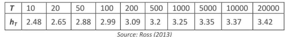
. (8) Ross (2013) provides simulated critical values hT for various T’s, as see i Ta le 1 below.
Table 1: Simulated critical values for NPCPM testing procedure
T 10 20 50 100 200 500 1000 5000 10000 20000
hT 2.48 2.65 2.88 2.99 3.09 3.2 3.25 3.35 3.37 3.42 Source: Ross (2013)
Again, if MT > hT then a structural break is discovered, and the best estimate of that break moment is
|
|
max
arg
ˆ
k kD
38
Firstly, we will perform the three detection techniques: ICSS, NPCPM and Cheng algorithm upon simulated data. Specifically, conditionally Gaussian Threshold-GARCH multiplicative models are considered with single and then multiple volatility breaks.
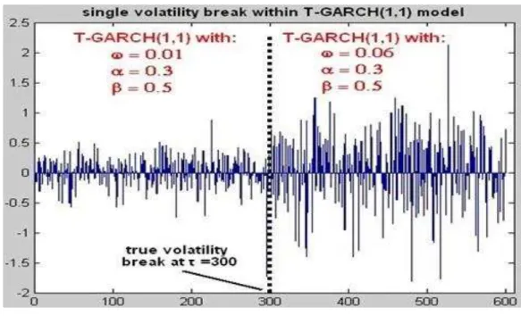
The first model to be examined below is T-GARCH(1,1) with single structural break at τ = 300, namely, for
600
1
t
T
600
300
;
5
.
0
3
.
0
06
.
0
300
1
;
5
.
0
3
.
0
01
.
0
2 1 2 1 2 1 2 1 2t
R
t
R
R
t t t t t t t t
(9)where innovations ɛt ~ iid N(0,1) and
{
1}
2 2
t tt
E
R
is a conditional variance, adapted to the process filtration
t
{
R
s:
s
t
}
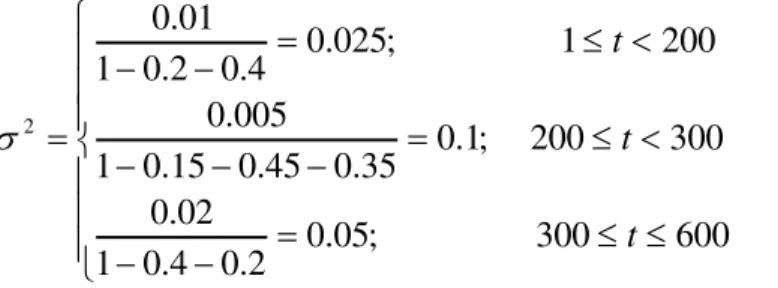
. (9) is just a concatenation of two separate, wide-sense stationary GARCH(1,1)models, introduced and explored in Bollerslev (1986). Unconditional variance of Rt in (9) can be easily calculated and it contains evident structural break at τ = 300:
.
600
300
for
3
.
0
5
.
0
3
.
0
1
06
.
0
300
1
for
05
.
0
5
.
0
3
.
0
1
01
.
0
2 2t
t
ER
t
(10)Figure 3 presents the simulated path together with the break at half-time.
Figure 3: Simulated path of T-GARCH(1,1) model (9), T=600, with single volatility break at =300
39
All the three detection techniques identified the change-point time with satisfactory accuracy. Both ICSS and NPCPM produced
ˆ
295
, hile Che g’s de i e ga e
ˆ
299
and similarly proper results were reported for other piecewise weakly stationary T-GARCH(1,1) models with various structural break location, as soon as it is not too close to series start or end.Next, we consider a simulated conditionally Gaussian, varying size T-GARCH model with two distinct volatility breaks. Specifically,
GARCH(1,1)
600
300
;
2
.
0
4
.
0
02
.
0
GARCH(2,1)
300
200
;
35
.
0
45
.
0
15
.
0
005
.
0
ARCH(2)
200
1
;
4
.
0
2
.
0
01
.
0
2 1 2 1 2 2 2 1 2 1 2 2 2 1 2t
R
t
R
t
R
R
R
t t t t t t t t t t t
(11)
This is again a piecewise weakly stationary GARCH model in which unconditional variance has two breaks at points predetermined in (11), and the calculus goes similarly as in (10):
600
300
;
05
.
0
2
.
0
4
.
0
1
02
.
0
300
200
;
1
.
0
35
.
0
45
.
0
15
.
0
1
005
.
0
200
1
;
025
.
0
4
.
0
2
.
0
1
01
.
0
2t
t
t
(12)The volatility (measured by variance) jumps four-fold at first breakpoint and halves its intensity at second breakpoint. The simulated trajectory of (11) is presented in Figure 4.
Figure 4: Simulated path of T-GARCH model (11), T=600, with 2 breaks at 1=200, 2=300
40
The break detection results obtained by using each of the employed algorithms are the following:
Table 2: The algorithms performance on simulated T-GARCH model with 2 volatility breaks
algorithm true τ’s estimated
ˆ
'
s
ICSS
200; 300
194; 295
Cheng 194; 218; 292; 310; 431
NPCPM 194; 295
Source: Autho ’s own computations
ICSS and NPCPM work satisfactorily well, detecting breaks close to the true ones. However, the performance of the Cheng algorithm for multiple volatility breaks is highly disputable. Too many points have been flagged, either due to fat tails or the issue of its applicability for multiple break detection (which seems to have remained an open question, in the above simulations answered negatively). Therefore at this stage, in analysis of real financial time series we discard this algorithm, restricting ourselves to comparing the remaining two.
Finally, we proceed to volatility break detection within logreturns of the two stock indices mentioned in Section 2, namely DAX30 and S&P500, see Figure 1. Both series consist of roughly T=4650 observations, which encompass alternate periods of prosperity, boom (markets in complacency mode), followed by bust/crash and resulting recession (markets in high nervousness regime). We compare numerical performance of ICSS and NPCPM techniques on these real data, exhibiting leptokurticity, serial dependence, possibly long memory and sudden profound regime changes caused by external shocks of great magnitude.
Figures 5 and 6 present the final results of volatility break detection, carried out on {Rt}, but for graphical convenience superimposed on daily indices quotes series {St}, see (1).
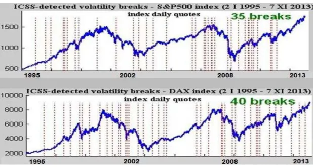
Figure 5: Detection of structural breaks in S&P500 and DAX30 indices: ICSS algorithm
41
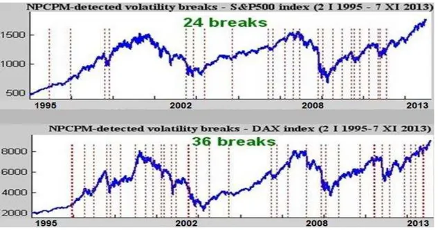
Figure 6: Detection of structural breaks in S&P500 and DAX30 indices: NPCPM algorithm
Source: Autho ’s own computations and graph based on data acquired from www.bossa.pl
The ICSS algorithm looks over-sensitive, largely due to violation of the rigorous assumptions in I&T (1994), discussed above. 35 structural breaks in the US case and 40 in Germany translate into roughly half-yearly volatility breaks, but the detected change points cluster on the time line. The signals tend to appear with larger intensity during severe bear markets and higher uncertainty implied by considerable deviations of logreturns. In contrast, stable bull markets produce scarcer breaks, eg. not a single one has been recorded on the S&P500 within more than a one-year horizon until the series terminates on Nov 7, 2013. The DAX index itself is more volatile, hence more breaks are recorded. This may be partly explained by the ongoing economic instability of several eurozone countries. In both cases however, NPCPM proves more robust – we have 24 breaks in US and 36 in German financial volatility. Disappointingly, the algorithm has not captured the onset of the post-dotcom-bubble recession in the USA, staying blind until 2002.
Detecting structural breaks in volatility is a challenging task, solved with various efficiency by several authors, under their specific sets of model assumptions. We compared three such algorithms of break detection for a simulated hypothetical return series and main stock indices. In general they perform better under a single break or when these regime changes are rare. ICSS technique is found to be quite sensitive to outliers, while NPCPM is more robust, ignoring some spurious breaks. Che g’s de i e also overreacts to outliers. A single structural break is detected satisfactorily by all methods, provided lack of severe outliers within the data. Iterative versions of some techniques prove sometimes questionable, which was shown in our simulations. Specifically, successive iterations of Cheng’s algorithm beyond true breaks flag false signals. This suggests that the iterative version of the method does not converge, so the technique is suitable for detection of a single or at best two breaks. Ross’ device is not fully autonomous as it i he its so e of the breaks detected by ICSS.
42
dynamics) mainly induced only by the heavy tails of logreturns series. Indeed, in financial econometrics, the time series structure is much more complicated (seasonalities, dummy effects, long memory, skewness, etc.), therefore the break signals are noisy and not always trustworthy. To produce more precise, de-noised techniques of volatility break detection, multivariate modelling could be advocated. More precisely, some explanatory additional time series like e.g. large fund cashflows, intensity of monetary interventions, margin debt levels and aggregate measures of investment sentiment might be used to enhance the detection probability of proper, long-lasting regime change, also for a wider scope of quotable assets than presented above. Discerning between endogenous and exogenous shocks would be helpful, too.
There still seems to be vast space for further research, aiming at more proper volatility structural break detection techniques. Multivariate time series analysis with some exogenous processes (like global sentiment indicators and the s ale of o eta y ua titati e easi g ) could substantially improve statistical inference, but at the evident cost of far more complex theoretical setup and simulations. The ongoing financial turbulence of the recent decade gives a strong motivation for further exploration of models with structural breaks in volatility. Proper detection of crucial breaks vitally enhances statistical inference in financial time series, see e.g. Covarrubias et al. (2006), Kang, Cho and Yoon (2009). On that basis (in practice, real-time break detection is very welcome) one can separately model the series’ dynamics within distinct regimes, separated by the discovered break times. The present, prolonged but artificially sustained complacency of the financial markets is not granted once for good.
The author would like to thank an anonymous referee for her/his helpful comments contributing especially to understanding the broader applicational potential of volatility break detection techniques, possibly in the context of a multivariate framework helping to identify the most important volatility breaks.
The paper is supported by the NCN grant UMO-2013/10/M/ST1/00096.
Aggarwal, R., I lá , C., Leal, R. (1999). Volatility in Emerging Stock Markets. Journal of Financial and Quantitative Analysis 34, 33–55.
Andreou, E., Ghysels, E. (2002). Detecting Multiple Breaks in Financial Market Volatility Dynamics. Journal of Applied Econometrics 17, 579–600.
Bollerslev, T. (1986). Generalized Autoregressive Conditional Heteroscedasticity. Journal of Econometrics 37, 307– 327.
Cheng, T. L. (2009). An Efficient Algorithm for Estimating a Change-point. Statistics and Probability Letters 79, 559– 565.
Covarrubias, G., Ewing, B. T., Hein, S. E., Thompson, M. A. (2006). Modeling Volatility Changes in the 10-year Treasury. Physica A 369, 737–744.
Eckley, I. A., Killick, R., Evans, K., Jonathan, P. (2010). Detection of Changes in Variance of Oceanographic Time-series Using Changepoint Analysis. Ocean Engineering 37, 1120-1126.
Inclán, C., Tiao, G. C. (1994). Use of Cumulative Sums of Squares for Retrospective Detection of Changes of Variance. Journal of the American Statistical Association 89, 913–923.
43
Kokoszka, P., Leipus, R. (2000). Change-point Estimation in ARCH Models. Bernoulli 6 (3), 513–539.
Mood, A. M. (1954). On the Asymptotic Efficiency of Certain Nonparametric Two-sample Tests. Annals of Mathematical Statistics 25(3), 514–522.
Rapach, D., Strauss, J. K. (2008). Structural Breaks and GARCH Models of Exchange Rate Volatility. Journal of Applied Econometrics 23, 65–90.
Ross, G. J. (2013). Modeling Financial Volatility in the Presence of Abrupt Changes. Physica A. Statistical Mechanics and its Applications 192(2), 350–360.
“a só, A., A agó, V., Carrion-i-Silvestre, J. L. (2004). Testing for Changes in the Unconditional Variance of Financial Time Series. Revista de Economia Financiera 4, 32–53.