Abstract—Microarray gene expression data generally suffers from missing values, which adversely affects downstream analysis. A new similarity metric method called reduced relational grade was proposed, based on which we further presented an improved KNN method named RKNN imputation algorithm for iteratively estimating microarray missing values. Reduced relational grade is an improvement of gray relational grade. The former can achieve the same performance as the latter, whereas the former can greatly reduce the time complexity. RKNN imputes missing data iteratively by considering the reduced relational grade as similarity metric and expanding the set of candidate genes for nearest neighbors with imputed genes, which increases the effect and performance of the imputation algorithm. We selected data sets of different kind, such as time series, mixed and non-time series, and then experimentally evaluated the proposed method. The results demonstrate that the reduced relational grade is effective and RKNN outperforms common imputation algorithms.
Index Terms—Gene expression data, reduced relational grade, imputation, iteration
I. INTRODUCTION
N important part of human genome project is to analyze and utilize microarray gene expression data, which records the abundance of gene transcripts mRNA in cells and contains significant control information about gene function. Microarray analysis technology on gene expression data has been widely used in numerous fields related to investigating drug effects, identification of critical genes for diagnosis or therapy and cancer classification.
DNA microarray technology [1] is one of the most useful tools for monitoring gene expression level, which can simultaneously analyze the mRNA levels of thousands of genes in particular cells or tissues on a gene chip. In a DNA microarray experiment, plenty of DNA probes are fixed on a given spot, and then hybridized with samples of fluorescence labeled DNA, cDNA or RNA, so the gene sequence information can be obtained by detecting the strength of
Manuscript received September 02, 2015; revised December 14, 2015. This work was supported in part by the National Natural Science Foundation of China (U1433116), the Fundation of Graduate Innovation Center in NUAA (kfjj20151602).
Yun He is with the College of Computer Science and Technology, Nanjing University of Aeronautics and Astronautics, Nanjing, 210016 China. (E-mail: [email protected]).
De-Chang Pi is with the College of Computer Science and Technology, Nanjing University of Aeronautics and Astronautics, Nanjing, 210016 China. (E-mail: [email protected]).
hybridization signal.
Even though microarray technology is efficient, accurate and low-cost, it still suffers from the problem of missing values due to a variety of internal or external factors in experiments. The missing value can account for 10% and even in some cases, up to 90% of genes have one or more missing values [2]. All of such issues as image corruption, hybridization failures, insufficient resolution, or dust and scratches on slide can cause gene missing values.
Many data analysis methods, such as principal component analysis (PCA), singular value decomposition (SVD) and hierarchical clustering, just can be applied with complete datasets without missing values. Besides, it has been found that missing values impede microarray data analysis and law discovery [4]. Experimenting repetitively is regarded as a way to solve missing data problem, but most of them are complex, costly and time-consuming. Deleting incomplete genes before analyzing is a simple approach to obtain a complete dataset. Unfortunately, deletion strategy omits incomplete genes, so it leads to insufficient original dataset especially for multivariate data like microarray gene expression. It generates serious bias and inaccurate conclusion when missing ratio is large or data distribution of missing values is non-random [5]. Missing value imputation [6]-[7] is a low-cost and efficient approach to recover all missing data without repetitive experiments [8]. Substituting missing values with the global or class-conditional mean/mode has been employed to handle missing values. Furthermore, imputation before analysis can significantly improve the performance of some machine learning algorithms which suffer missing values, namely C4.5, reference [9] shows that KNN imputation can enhance prediction accuracy of C4.5 over small software project datasets.
We propose an iterative imputation algorithm based on a kind of novel distance metric for predicting gene expression missing values, called Iterative imputation based on reduced relational grade (RKNN). RKNN measures the similarity between a gene with missing values and its nearest neighbors with the reduced relational grade, which improves gray relational grade. Besides, imputing missing values iteratively has high data utilization by using incomplete genes (with missing values). We experimentally evaluate the proposed algorithm on different kinds of publicly available microarray datasets and the results demonstrate that the reduced relational grade achieve similar performance as gray one
when capturing ‘nearness’ but greatly reduces the time
complexity. Moreover, RKNN algorithm outperforms the
Improving KNN Method Based on Reduced
Relational Grade for Microarray Missing Values
Imputation
Yun He, De-chang Pi
conventional KNN method.
The rest of this paper is organized as follows. It has a brief review on related work about imputation methods in Section II. In Section III, we introduce the concept of gray relational grade. Both the reduced relational grade and RKNN algorithm are proposed in Section IV, while the analysis of them are discussed in Section V. In Section VI we conclude this paper.
II. RELATED WORK
Throughout this paper, the original gene expression matrix (with missing values) is denoted byX , which contains n genes and m attributes (n m), where the i-th row represents gene xi and xi[x xi1, i2, ,xim]. xij denotes the expression
level of genexi in sample j. All of complete genes from X constitute a complete data matrix complete
X (without missing values). The gene with missing values is called a target gene, and the set of genes with available information for imputing missing values in a target gene is referred as its candidate genes.
K nearest-neighbors (KNN) imputation is defined to find K nearest neighbors from complete data sets for the target gene assumed to have a missing value in attribute j, and then fill in the target gene with a weighted average of values in attribute j from the K closest genes [10]. The idea of KNN is that objects close to each other are potentially similar. For a gene expression dataset, similar genes in similar experiments will have similar expression, based on which KNN implements the imputation for gene expression datasets.
Reference [10] presented a comparative study of three kinds of imputation methods, namely Singular Value Decomposition-based method, KNN and row average, on gene microarray data of different missing ratio. Experimental results showed that KNN imputation has the best robustness and accuracy. Reference [11] synthetically analyzed the performances of 23 kinds of imputation methods and demonstrated that KNN imputation has excellent estimation accuracy. So far, many researches have improved KNN imputation and they mainly aim at two aspects: the order of imputation and the metric distance. Among these researches, a sequential KNN (SKNN) imputation [12] method sorts the target genes (with missing values) according to their missing ratio and then imputes genes with the smallest missing rate first. Once all missing values in a target gene are imputed, the target gene will be considered as a complete one. Shell Neighbors imputation [13] fills in an incomplete instance by only using its left and right nearest neighbors with respect to each attribute, and the size of the set of nearest neighbors is determined by cross-validation method. Existing KNN imputation is based on Minkowski distance, which is a simple superimposed distance on different attributes of two genes without considering the whole data set. Reference [14] showed that gray relational grade is more appropriate to capture the proximity between two instances than Minkowski distance or others.
Single imputation that affords single estimation for each missing data is a kind of common strategy. Nevertheless, single imputation cannot provide effective standard errors and
confidence intervals because it ignores the uncertainty of the imputed dataset [14]-[15]. Filling in missing values with iterative imputation is the alternative of single imputation. Reference [16] presented a nonparametric iterative imputation algorithm and confirmed that it outperforms normal single imputation. Iterative imputation based on gray relational grade (GKNN) proposed in [14] uses gray relational grade as its similar metric to select K nearest neighbors. GKNN can obtain great results when dealing with missing values in heterogeneous data (continuous and discrete data). However, GKNN is more suitable for small datasets, because calculating the grey correlation degree costs a lot of time with the expansion of the data scale. We propose a RKNN imputation algorithm based on GKNN in this paper, and reduced relational grade is designed as the similar metric method, which can significantly decrease time complexity and keep the good imputation performance compared with the conventional relational grade.
III. GRAY RELATIONAL GRADE
Gray System Theory (GST) was developed by Deng in 1982 [17]. The System is good at handling complex systems to get reliable results. Gray Relational Analysis (GRA), a method of GST, can seek the numerical relationship among different subsystems to measure the similarity. GRA is used to quantify the trend relationship of two systems or two elements in a system. Generally, if the development tendency between two systems is consistent, the relational grade is large. Otherwise, it is small.
Gray relational coefficient (GRC) is used to describe the similarity between a target and a candidate gene on the attribute q in a given dataset.xi andxj represent the target
and the candidate gene respectively. The GRC is defined as follows:
min min | x x | max max | x x | (x , x )
| x x | max max | x x |
t k ik tk t k ik tk
iq jq
iq jq t k ik tk
GRC
(1) where is the distinguishing coefficient, [0,1] , generally =0.5.
Gray relational grade takes mean processing to change each
series’ gray relational coefficient at all attributes into their average as similarity metric of two genes.
1
1
GRG(x , x ) (x , x )
m
i j ik jk
k
GRC m
(2) GRG measures the relationship between two genes at a global perspective, which overcomes the deficiency of Minkowski distance. When selecting K nearest neighbors for a target gene, the larger the value of gray relational grade is, the higher similarity and the less difference between genes are. Otherwise, the less similarity and the more difference.IV. RKNNALGORITHM
A. Reduced relational grade
experimental conditions. According to (1), we must search the whole candidate dataset one time when calculating a GRC of each target gene. For gene data matrix, this kind of approach will cost too much time. In this paper, we propose a new relational coefficient denoted as Reduced Relational Coefficient (RRC), which is a kind of reduce of GRC. RRC is appropriate for measuring the nearness between a target genexi and a candidate genexjat a specific attributes q:
{ x min , x max }
(x , x )
x x { x min , x max }
k ik k ik k
iq jq
iq jq k ik k ik k
Max RRC Max
(3)
Where functionMax{,}takes the larger one of two values.
mink and maxk refer to the minimum and maximum values of attributes k respectively, which are easily obtained during the process of data inputting or data normalizing.
With experimenting in many times, we found the calculation result of formula min mint k| xikx |tk always tends to zero, and the value of max maxt k| xikx |tk tends
toMaxk{| xikmin |,| xk ikmax |}k . In short, equation (3) is
a simplification of (1), and that means the results of
min mint k | xikx |tk and max maxt k| xikx |tk , which
need a huge amount of computations, are approximately replaced by their extreme, so RRC can greatly reduce the time complexity.
In (3), RRC(x , x )iq jq is valued in [0, 1]. The greater the value of RRC(x , x )iq jq is, the larger the similarity between xiq andxjq will be. If xiqxjq, RRC(x , x ) 1iq jq . On the contrary, if xiq andxjqhave completely different values on
attribute q, the value of RRC(x , x )iq jq is minimal. The
reduced relational grade between the target genexi and the
candidate gene xj is defined as follows:
1
1
RRG(x , x ) (x , x )
m
i j ik jk
k
RRC m
(4) Similarly, RRG is also the mean processing and the greater the RRG is, the larger similarity between genes is achieved.Assume that the size of candidate gene dataset is N*m. For any target gene, when calculating its GRG with all of genes in candidate dataset, the time complexity is O(N*N*m); while calculating the RRG, the time complexity is reduced to O(N*m). The improvement of time complexity is amazing, considering gene expression dataset isN m.
B. Imputation
For a given target genexi (the value ofxit is missing),
RKNN calculates the RRG(x , x )i j between xi and each
candidate genexj , then selects K most similar genes as its K
nearest neighbors and finally imputesxit with the weighted
average of its K neighbor genes at attribute t: 1
ˆ K
it k ik kt
y
w x (5) Wherewik is the weight of k-th neighbor genexk toxi.1
( , ) / K ( , )
ik i k k i k
w RRG x x
RRG x x (6)C. Data normalization
Generally, the similarity between two genes is dominated by attributes with greater magnitude units. To avoid the bias generated by unit difference and make the data processing convenient, data should be normalized before calculating the reduced relational grade for RKNN imputation algorithm. In this paper, we select Min-Max normalization. Original data will be normalized into [0,1]. Assume that max(t) and min(t) represent the maximum and minimum values on attribute t respectively, andxit is the expression value of genexi on
attribute t. Data is normalized as follows:
min(t) max(t) min(t)
it it
x x
(7)
D. RKNN algorithm design
RKNN uses RRG as similarity metric method to select K neighbors and iteratively imputes missing values with weighted average until the termination condition is satisfied.
expression missing expression mi : : : 01: : 02 : 03 g 04 s
: s in
i i RKNNimpute
gene dataset X with values complete gene dataset
x Initialization
FOR each target gene in X
replece all values inx withrow averages
Algorithm Input Output
Step1
( )0 : / / obtaining a complete matrix
06 : :
07 : 0
08 :
09 : / / 1, 2, 3
10 : ) : ( 11 , i complete complete complete
END FOR X
normalize X X Imputation h
REPEAT
h the kth iterative imputation h FOR each target
get
x gene in X construc Step2 05:
( 1) 12 :13 : ,
14 :
using (6)?
17 : / / obtai
miss nin i g ng complete h j i j comple i
t the candidate gene dataset based onX FOR each candidate gene
compute RRG END FOR
elect the K nearest genes
impute all values in equation x
x x
x
END FOR X
15: 16:
( )
( ) ( ) (h 1) ( )
2 ( ) ( ) (h 1)
1
)
1
(h
ˆ ˆ
y , y
1 ˆ ˆ
19 : (y y )
18 :
20 :
20 : ( maximum )
te h
complete h c h j j N h h j j ompl j ete h m N
FOR each imputation value X X
compute
END FOR
UNTIL or reach N the number of iteration
Herein, generally convergence accuracy is 3
10
and the maximum number of iteration isNm10.
The accuracy of imputation algorithm is evaluated by the root mean square error (RMSE) as follows:
2 1 ˆ (y ) N i i i y RMSE N
V. EXPERIMENTS AND ANALYSIS
A. Data
Gene expression data from microarray technology is a matrix, which presents of expression level of various genes (rows) under different experimental conditions (columns). In this study, we used five public available microarray data sets in three different types obtained from the public genetic databases: http://www.ncbi.nlm.nih.gov/geo/.
Two data sets (data sets NTS1 and NTS2) from the study in yeast Saccharomyces cerevisiae consist of non-time series microarray data. The NTS1 is a comparison of cDNA coming from mex67-5 temperature-sensitive mutant and that from Mex67 wildtype strain both at 37℃, while NTS2 compares cDNA from yra1-1 temperature-sensitive mutant with that from Yra1 wildtype strain both at 37℃ too. Both NS1 and NS2 have six samples representing six experiments.
The third and the fourth data sets (data sets TS1 and TS2) are time series data. TS1 tested the transcriptional response of S.cerevisiae to aeration after anaerobic growth. The six attributes of TS1 stands for how long it has been aerated. TS2 contains the data from a cdc15-2-based sychronisation, which is composed of 25 attributes implying different culture time. The fifth data set belongs to a study of gene expression in Salmonella enterica after treating with 2mM hydrogen peroxide. It is termed by MIX, and contains both time and non-time course data.
TABLE I
DIMENSION AND TYPES OF THE GENE EXPRESSION DATASETS
Data set
Original Data Complete Data Missing
Rate Type
row column row column
NTS1 7684 6 7106 6 1.46% non-time
series
NTS2 7684 6 7589 6 0.04% non-time
series
TS1 6495 6 3491 6 12.07% time
series
TS2 8832 25 4078 25 16.10% time
series
MIX 5184 6 5151 6 0.11 mixed
series
All of these five data sets suffer missing problems, especially TS2. Firstly, these data sets need to be pre-processed by removing genes with missing values to obtain complete data sets. Table I shows the dimensions of the original data matrices before and after pre-processing (complete data).
Before experimenting, missing values at different ratio were introduced into these five complete data sets randomly, and then they are analyzed by imputation algorithm.
B. Parameter K
KNN method or its variations have one thing in common: An appropriate K must be selected. The value of K can affect the prediction of KNN method or its variations. If K is too large, the similarity of some neighbors will be insufficient, and too much neighbors may result in imputation performance reduction; if K is too small, it will strengthen a few neighbors and the negative impact of noise data will increase simultaneously. The value of K is empirically found related to
the type of data and missing ratio, but in theory, there is no exact formula. Reference [18] designed a procedure for selecting K automatically, and demonstrated that K can be set to any value in the range 10-15. Reference [10] addressed this question in KNN method and reported the best results for K is in the range 10-20. It was fond experimentally that when K is valued in [10, 15], the fluctuation of K can hardly affect the performance of algorithms. Therefore, we take K=10 in subsequent experiments.
C. Experimental evaluation on RRG
In order to assess the performance of RRG, GRG was used as a reference. Whether RRG can improve the system property when compared with GRG was indirectly showed by the comparison results of RKNN and GKNN, since the only distinction of these two algorithms lies in different similarity metric methods.
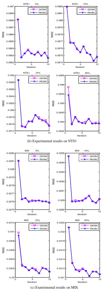
Comparison results are presented in Fig. 1, where Fig. 1(a) display the RMSE on TS1 dataset with missing ratio 5%, 10%, 15%, 20%, respectively. Similarly, Fig. 1(b) and Fig. 1(c) are the results on datasets NTS1 and MIX, separately.
The results show that the RMSE of the second iteration dramatically decreases when compared with the first iteration imputation both in RKNN and GKNN algorithms at different missing ratio. So iterative procedure can refine the imputation value. From Fig 1, the two curves, which describe the performance of RKNN and GKNN, basically coincide in each subfigure. That indicates the two imputation algorithms based on RRG and GRG approximately have the same imputation accuracy, which means that considering neighbors selection and weight calculation, the same results as GRG are achieved by applying RRG as the similarity metric.
0 5 10 0.0465
0.047 0.0475 0.048 0.0485 0.049
Iteration
R
M
S
E
TS1 5%
0 5 10 0.048
0.0482 0.0484 0.0486 0.0488 0.049 0.0492 0.0494 0.0496
Iteration
R
M
S
E
TS1 10%
GKNN RKNN
GKNN RKNN
0 5 10 0.0515
0.052 0.0525 0.053 0.0535 0.054 0.0545 0.055 0.0555 0.056
Iteration
R
M
S
E
TS1 15% GKNN RKNN
0 5 10 0.053
0.054 0.055 0.056 0.057 0.058 0.059
Iteration
R
M
S
E
TS1 20%
GKNN RKNN
0 5 10 0.0862
0.0863 0.0864 0.0865 0.0866 0.0867 0.0868 0.0869 0.087
Iteration
R
M
S
E
NTS1 5% GKNN RKNN
0 5 10 0.0874
0.0875 0.0876 0.0877 0.0878 0.0879 0.088 0.0881 0.0882
Iteration
R
M
S
E
NTS1 10% GKNN RKNN
0 5 10 0.0914
0.0916 0.0918 0.092 0.0922 0.0924 0.0926 0.0928 0.093
Iteration
R
M
S
E
NTS1 15%
GKNN RKNN
0 5 10 0.0935
0.094 0.0945 0.095 0.0955 0.096 0.0965
Iteration
R
M
S
E
NTS1 20%
GKNN RKNN
(b) Experimental results on NTS1
0 5 10 0.0275
0.0276 0.0277 0.0278 0.0279 0.028 0.0281 0.0282
Iteration
R
M
S
E
MIX 5% GKNN RKNN
0 5 10 0.0289
0.029 0.0291 0.0292 0.0293 0.0294 0.0295
Iteration
R
M
S
E
MIX 10% GKNN RKNN
0 5 10 0.03
0.0302 0.0304 0.0306 0.0308 0.031 0.0312
Iteration
R
M
S
E
MIX 15%
GKNN RKNN
0 5 10 0.031
0.0312 0.0314 0.0316 0.0318 0.032 0.0322
Iteration
R
M
S
E
MIX 20%
GKNN RKNN
(c) Experimental results on MIX
Fig. 1. Experimental results for ten iterations on TS1, NTS1 and MIX datasets for RKNN and GKNN algorithms.
Table II presents time-consuming scale of the comparison experiments on dataset TS1, similarly Table III and Table IV display the time-consuming of RKNN and GKNN on dataset NTS1 and dataset MIX, respectively. Obviously, RRG proposed in this paper compared with GRG can decrease computational complexity significantly, and reduce runtime
effectively as well.
TABLE II
TIME-CONSUMING OF RKNN AND GKNN FOR TEN ITERATIONS ON TS1
Consuming
time (ms) Dataset TS1
missing ratio 5% 10% 15% 20%
RKNN 2978 5388 6876 8096
GKNN 4111439 7176826 8904707 11435077
TABLE III
TIME-CONSUMING OF RKNN AND GKNN FOR TEN ITERATIONS ON NTS1
Consuming
time (ms) Dataset NTS1
missing ratio 5% 10% 15% 20%
RKNN 11582 21032 28565 31979
GKNN 33457400 60015902 79448905 96778006
TABLE IV
TIME-CONSUMING OF RKNN AND GKNN FOR TEN ITERATIONS ON MIX
Consuming
time (ms) Dataset MIX
missing ratio 5% 10% 15% 20%
RKNN 6185 10925 13945 18185
GKNN 14534205 23306022 29330607 36188027
Overall, RRG has same performance as GRG on imputation accuracy. Moreover, RRG greatly reduces the time complexity.
D. Experimental evaluation on RKNN
In order to evaluate the proposed RKNN algorithm with some microarray data sets, two algorithms were selected in our experiments. One is the algorithm of sequential KNN imputation (SKNN), the other is the iterative KNN imputation (IKNN) [17] by changing normal KNN method into an iterative imputation based on iterative principle.
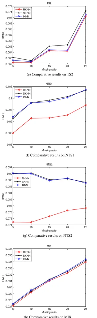
RKNN, SKNN and IKNN are applied to five datasets TS1, TS2, NTS1, NTS2, and MIX at different missing ratio 5%, 10%, 15%, 20% and 25%. The experimental results in RMSE showed the phenomenon of prediction accuracy for these three imputation algorithms in Fig 2.
(d) Comparative results on TS1
5 10 15 20 25
0.048 0.05 0.052 0.054 0.056 0.058 0.06 0.062 0.064
Missing ratio
R
M
S
E
TS1
5 10 15 20 25 0.062
0.063 0.064 0.065 0.066 0.067 0.068 0.069 0.07 0.071 0.072
Missing ratio
R
M
S
E
TS2
RKNN SKNN IKNN
(e) Comparative results on TS2
5 10 15 20 25
0.08 0.085 0.09 0.095 0.1 0.105
Missing ratio
R
M
S
E
NTS1
RKNN SKNN IKNN
(f) Comparative results on NTS1
5 10 15 20 25
0.074 0.076 0.078 0.08 0.082 0.084 0.086 0.088 0.09 0.092
Missing ratio
R
M
S
E
NTS2
RKNN SKNN IKNN
(g) Comparative results on NTS2
5 10 15 20 25
0.027 0.028 0.029 0.03 0.031 0.032 0.033 0.034 0.035 0.036
Missing ratio
R
M
S
E
MIX
RKNN SKNN IKNN
(h) Comparative results on MIX
Fig. 2. Experimental results on datasets TS1, TS2, NTS1, NTS2 and MIX for three algorithms.
From Fig 2, we find that the accuracies of algorithms
decrease while the missing ratio increases generally. Fig. 2(d), Fig. 2(e) and Fig. 2(h) presented the results on time series datasets TS1, TS2, and mixed dataset MIX, respectively. The imputation accuracies of RKNN, SKNN and IKNN are close to each other over these three datasets, but we can still find out that RKNN has the smallest estimation error. The advantage of RKNN is very obvious on non-time series datasets NTS1 and NTS2 displayed in Fig. 2(f) and Fig. 2(g). The performance of algorithms depends on the type of datasets, and RKNN is more appropriate for non-time series datasets. Hence, compared with IKNN and SKNN algorithms, our method RKNN has the best performance.
VI. CONCLUSIONS
In this work, we proposed a new similarity metric method named reduced relational grade (RRG), which is an improvement of GRG. The performance of RRG was indirectly assessed and compared with GRG over three datasets of different types at different missing ratio. Considering estimation accuracy, RRG and GRG have the same similar results, but RRG significantly decreases the time complexity. Therefore, RRG is a kind of more efficient
method to capture ‘nearness’ between two instances
compared with GRG. Based on RRG, we further proposed an improved KNN method for estimating missing values on microarray gene expression data, named RKNN imputation. RKNN is ability to efficiently utilize data and it also can impute missing values iteratively. We experimentally evaluated the performance of RKNN compared with IKNN and SKNN algorithms on five datasets at different missing ratio. The results show that RKNN works well on imputing missing values. It should also be noted that the appropriate convergence accuracy and the maximum number of iteration can affect the performance of RKNN imputation, so how to efficiently and reasonably determine them would be further researched.
REFERENCES
[1] Hoheisel J D. “Microarray technology: beyond transcript profiling and
genotype analysis,” Nature Reviews Genetics, vol. 7, no. 3, pp.
200-210, 2006.
[2] Brevern A G D, Hazout S, Malpertuy A. “Influence of microarrays experiments missing values on the stability of gene groups by
hierarchical clustering,” BMC Bioinformatics, vol. 5, no. 1, pp. 114-119, 2004.
[3] Yang Y H, Buckley M J, Dudoit S, et al. “Comparison of methods for
image analysis on cDNA microarray data,” Journal of Computational and Graphical Statistics, vol. 11, no. 1, pp. 108-136, 2002.
[4] Junger W L, de Leon A P. “Imputation of missing data in time series for
air pollutants,” Atmospheric Environment, vol. 102, pp. 96-104, Feb 2015.
[5] García-Laencina P J, Sancho-Gómez J L, Figueiras-Vidal A R, et al. “K nearest neighbours with mutual information for simultaneous
classification and missing data imputation,” Neurocomputing, vol. 72, no. 7-9, pp. 1483-1493, 2009.
[6] Fukuta K, Okada Y. “LEAF: Leave-one-out Forward Selection method
for information gene discovery in DNA microarray data,” IAENG
International Journal of Computer Science, vol. 38, no. 2, pp 160-167, 2011.
[7] Okada Y, Okubo K, Horton P, et al. “Exhaustive search method of gene
expression modules and its application to human tissue data,” IAENG
[8] Moorthy K, Saberi Mohamad M, Deris S. “A Review on Missing Value Imputation Algorithms for Microarray Gene Expression Data,”
Current Bioinformatics, vol. 9, no. 1, pp. 18-22, 2014.
[9] Song Q, Shepperd M, Chen X, et al. “Can k-NN imputation improve the performance of C4.5 with small software project data sets? A
comparative evaluation,” The Journal of Systems and Software, vol. 81, no. 12, pp. 2361-2370, 2008.
[10] Troyanskaya O, Cantor M, Sherlock G, et al. “Missing value
estimation methods for DNA microarrays,” Bioinformatics, vol. 17, no. 6, pp. 520-525, 2001.
[11] Liew A W C, Law N F, Yan H. “Missing value imputation for gene expression data: computational technique to recover missing data from
available information,” Briefings in Bioinformatics, vol. 12, no. 5, pp. 498-513, 2010.
[12] Meng F, Cai C, Yan H. “A Bicluster-Based Bayesian Principal Component Analysis Method for Microarray Missing Value
Estimation,” Biomedical and Health Informatics, vol. 18, no. 3, pp. 862-871, 2014.
[13] Zhang S. “Shell-neighbor method and its application in missing data,”
Applied Intelligence, vol. 35, no. 1, pp. 123-133, 2011.
[14] Zhang S. “Nearest neighbor selection for iteratively KNN imputation,”
The Journal of Systems and Software, vol. 85, no. 11, pp. 2541-2552, 2012.
[15] Riggi S, Riggi D, Riggi F. “Handling missing data for the identification of charged particles in a multilayer detector: A comparison between
different imputation methods,” Nuclear Instruments and Methods in
Physics Research A, vol. 780, pp 81-90, Apr 2015.
[16] Zhang S, Jin Z, Zhu X. “NIIA: Nonparametric Iterative Imputation
Algorithm”, Berlin: Springer-Verlag, 2008.
[17] Song Q, Shepperd M. “Predicting software project effort: A grey
relational analysis based method,” Expert Systems with Applications. vol. 38, no. 6, pp. 7302-7316, 2011.
[18] Brás L P, Menezes J C. “Improving cluster-based missing value