www.hydrol-earth-syst-sci.net/19/1469/2015/ doi:10.5194/hess-19-1469-2015
© Author(s) 2015. CC Attribution 3.0 License.
Operational river discharge forecasting in poorly gauged basins:
the Kavango River basin case study
P. Bauer-Gottwein1, I. H. Jensen1, R. Guzinski2, G. K. T. Bredtoft1, S. Hansen1, and C. I. Michailovsky1,3 1Department of Environmental Engineering, Technical University of Denmark, 2800 Kgs. Lyngby, Denmark 2DHI GRAS, 2970 Hørsholm, Denmark
3now at: Jet Propulsion Laboratory, California Institute of Technology, Pasadena, California, USA Correspondence to:P. Bauer-Gottwein ([email protected])
Received: 5 September 2014 – Published in Hydrol. Earth Syst. Sci. Discuss.: 8 October 2014 Revised: 2 March 2015 – Accepted: 3 March 2015 – Published: 23 March 2015
Abstract. Operational probabilistic forecasts of river dis-charge are essential for effective water resources manage-ment. Many studies have addressed this topic using dif-ferent approaches ranging from purely statistical black-box approaches to physically based and distributed modeling schemes employing data assimilation techniques. However, few studies have attempted to develop operational probabilis-tic forecasting approaches for large and poorly gauged river basins. The objective of this study is to develop open-source software tools to support hydrologic forecasting and inte-grated water resources management in Africa. We present an operational probabilistic forecasting approach which uses public-domain climate forcing data and a hydrologic– hydrodynamic model which is entirely based on open-source software. Data assimilation techniques are used to inform the forecasts with the latest available observations. Forecasts are produced in real time for lead times of 0–7 days. The oper-ational probabilistic forecasts are evaluated using a selection of performance statistics and indicators and the performance is compared to persistence and climatology benchmarks. The forecasting system delivers useful forecasts for the Kavango River, which are reliable and sharp. Results indicate that the value of the forecasts is greatest for intermediate lead times between 4 and 7 days.
1 Introduction
Operational probabilistic hydrological modeling and river discharge forecasting is an active research topic in water re-sources engineering and applied hydrology (Pagano et al.,
2014). Sharp and reliable forecasts of river discharge are re-quired over a range of forecasting horizons for flood and drought management. A state of the art river discharge fore-casting system consists of a weather forecast or an ensem-ble of weather forecasts (Cloke and Pappenberger, 2009), a hydrologic–hydrodynamic modeling system and a data as-similation approach to inform the forecasts with all available in situ and remote sensing observations. Alternatively, in the absence of resources, data and computing power, simpler so-lutions can be implemented which disregard more and more of the physics and rely on past observations to parameterize black-box-type models such as, for instance, artificial neural networks (Maier et al., 2010).
Gaus-sian model errors. Variational data assimilation has also been used in a number of hydrologic studies (e.g., Seo et al., 2003, 2009). Some studies use filtering approaches where the gain is determined heuristically from offline simulations and then used operationally in forecasting mode (Madsen and Skotner, 2005). As pointed out by Liu et al. (2012), despite the large body of literature on hydrologic data assimilation, few stud-ies evaluate the benefit of data assimilation for actual fore-casting and practical application of data assimilation by op-erational agencies is rare.
In many river basins the performance of operational hy-drological modeling and forecasting is limited because in situ observations of precipitation and river discharge are scarce or unavailable. This is also the case for many of Africa’s large river basins which are poorly gauged (e.g., Zambezi, Volta, Congo). Consistent, long-term and spatially resolved in situ observations of precipitation and river discharge are unavail-able for large portions of Africa. Moreover, the number of operational meteorological stations and river discharge sta-tions has been decreasing consistently around the world since the 1970s (Fekete and Voeroesmarty, 2007; Peterson and Vose, 1997). Remote sensing techniques have the potential to fill critical data gaps in the observation of the global hydro-logical cycle. All major components of the water balance, ex-cept river discharge, can now be estimated based on various types of remote sensing data. However, the available tech-niques are still limited by coarse spatial and temporal reso-lution as well as large and/or poorly understood error char-acteristics (Tang et al., 2009). From a management perspec-tive one of the most important components of the hydrolog-ical cycle is river discharge. Extremely high flows in rivers cause flooding which can have severe consequences in terms of fatalities and economic damage. Low flows cause con-flicts in the allocation of scarce water resources between eco-nomic sectors and/or the environment. Therefore, in many river basins there is a need for hydrological models to provide operational estimates of river discharge based on remotely sensed observations and limited available in situ measure-ments.
The TIGER-NET project addresses the demand for free, up-to-date and spatially resolved water information for the African continent. The project is funded by the European Space Agency (ESA) and aims to support integrated water resources management in Africa by (i) providing access to ESA Earth observation (EO) data, (ii) developing an open-source Water Observation and Information System (WOIS) and (iii) implementing capacity building actions in collabora-tion with African partner institucollabora-tions (Guzinski et al., 2014). The WOIS includes a hydrological modeling component, which supports long-term scenario analysis (e.g., impact of climate change and deforestation) as well as operational probabilistic forecasting. The specific objective for the op-erational modeling capability is to provide reliable and sharp probabilistic forecasts of river discharge over time horizons of up to 1 week. In addition to hydrological modeling, WOIS
includes functionality for operational flood monitoring, basin characterization at high (∼30 m) and medium (∼1 km) spa-tial resolutions and derivation of other products requiring EO data processing and analysis (Guzinski et al., 2014). It was designed for use in African organizations, where budgetary and technical constraints often limit the use of EO data for integrated water resources management. Therefore, WOIS is based purely on free, open-source software components and was created as an easy-to-use tool for both capacity building and operational use. Among the partner institutions engaged in the TIGER-NET project is the Namibian Ministry of Agri-culture, Water and Forestry. The Ministry has an interest in forecasting the discharge of the Kavango River.
Based on these requirements, this study has four specific objectives:
1. development of a robust and simple probabilistic river discharge forecasting system for poorly gauged river basins, based solely on open-source software and public-domain data;
2. informing the forecasting system with in situ discharge observations in real time;
3. operational demonstration of the system for the Ka-vango River case study;
4. comprehensive evaluation of the operational probabilis-tic forecasts using a selection of performance statisprobabilis-tics and indicators as well as comparison with persistence and climatology benchmarks.
The entire system has been implemented in an open-source GIS environment (QGIS, GDAL, Python). Installation and source code are available for download from the TIGER-NET webpage (www.tiger-net.org).
2 Materials and methods
2.1 Study area
Figure 1.Base map for the Kavango River basin with location of in situ discharge stations. The coordinate system is UTM 33S, WGS84 datum. Inset map shows the location of the basin in southern Africa.
have been in focus for some time, flood risk has recently be-come a major concern because the northern part of Namibia has experienced increased magnitude and frequency of flood-ing events since 2008 (Wolski et al., 2014). Water managers need accurate and reliable forecasting tools to deal with both floods and droughts.
Three hydrological modeling efforts have been reported in the literature for the Kavango River basin. Folwell and Farqhuarson (2006) used the Global Water Availability As-sessment (GWAVA) model to assess climate change impacts in the basin. Hughes et al. (2006, 2011) calibrated a Pit-man model for the basin and were able to reproduce in situ observations satisfactorily. Milzow et al. (2011) developed a SWAT (Soil and Water Assessment Tool) model of the Kavango Basin and calibrated the model with water levels from radar altimetry, soil moisture from Envisat-ASAR (Ad-vanced Synthetic Aperture Radar) and total water storage change from GRACE (Gravity Recovery and Climate Exper-iment).
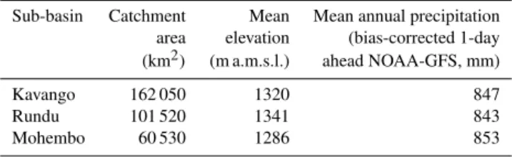
Long-term in situ observations of river discharge are avail-able from two hydrometric stations in the basin, Rundu and Mohembo (Fig. 1). Table 1 summarizes the main characteris-tics of the Kavango River basin and the two sub-basins con-tributing to the stations Rundu and Mohembo.
2.2 Hydrologic and hydrodynamic modeling
The modeling approach implemented in this study consists of a hydrologic (rainfall-runoff) model which is coupled to a
Table 1.Characteristics of the Kavango River basin and the Rundu and Mohembo sub-basins.
Sub-basin Catchment Mean Mean annual precipitation
area elevation (bias-corrected 1-day
(km2) (m a.m.s.l.) ahead NOAA-GFS, mm)
Kavango 162 050 1320 847
Rundu 101 520 1341 843
Mohembo 60 530 1286 853
simple routing model for channel flow. A one-way coupling between the two model compartments is implemented; i.e., once runoff has entered the river channel, the water cannot move back into the land phase of the hydrological cycle.
We use the well-known SWAT hydrological model, ver-sion 2009 (Gassman et al., 2005; Neitsch et al., 2011), for rainfall-runoff modeling. SWAT is a semi-distributed, phys-ically based hydrological model which operates at a daily time step. The river basin is divided into a number of sub-basins. Each sub-basin is in turn divided into hydrological response units (HRUs), which are defined as portions of the sub-basin with similar terrain slope, land use and soil type. The Kavango SWAT model consists of 12 sub-basins with outlets located at the confluences of major tributaries as well as at in situ discharge station locations (Fig. 1).
The hydrodynamic model used in this study is a simple Muskingum routing scheme, which is implemented outside of the SWAT simulator to allow efficient updating in the data assimilation scheme. Muskingum parameters are computed from river widths, assumed cross-section geometry and chan-nel Manning numbers (which are calibration parameters). The river is divided into 12 primary individual river reaches. The primary reaches are further subdivided if required to meet the numerical stability criteria of the Muskingum rout-ing scheme (Chow et al., 1988). The hydrodynamic model state vector consists of the simulated discharges in each indi-vidual reach. In the Muskingum routing scheme, the model operator propagating the discharge forward in time is linear; i.e., the simulated discharges at time stept+1 are a linear function of the simulated discharges at time stept and the runoff forcings at time stepstandt+1:
qt+1
=Aqt+Brt+Crt+1.
(1) In this equation,q is the vector of simulated discharges andr is the vector of runoff forcings,A,B andCare lin-ear operators which depend on the configuration of the river channels and network connectivity and the superscripts in-dicate time steps. For details on the implementation of the Muskingum routing scheme the reader is referred to Chow et al. (1988) and Michailovsky et al. (2013).
2.3 Input data
Table 2.Model performance for calibration and validation periods. Numbers in brackets are the percentage of mean observed flow.
In situ station NSE (–) RMSE (m3s−1) ME (m3s−1) Mean of No. of
observations (m3s−1) simulated observations Calibration period (2005–2011)
Rundu 0.73 105.6 (42.5 %) −5.4 (−2.2 %) 248.4 2440 Mohembo 0.69 97.1 (32.8 %) 6.8 (2.3 %) 295.9 1935
Validation period (2012–2014)
Rundu 0.74 94.6 (35.0 %) −55.0 (−20.6 %) 249.0 572 Mohembo 0.33 144.0 (30.7 %) −119.0 (−25.4 %) 469.1 46
used for automatic watershed and river network delineation as well as for the determination of terrain slope. We use the ACE2 (Altimeter Corrected Elevation, version 2; Berry et al., 2010) global elevation data set at a resolution of 30 arcsec. The parameterization of vegetation processes in the SWAT model is based on the land cover input data set. We use the USGS Global Land Cover Characterization (GLCC) data set, version 2.0 with a spatial resolution of 1 km (USGS, 2008). The soil data set forms the basis for parameterizing soil hy-draulic processes in SWAT. We use the FAO-UNESCO dig-ital soil map of the world and derived soil properties, revi-sion 1, with a spatial resolution of 5 arcmin (FAO-UNESCO, 1974). Look-up tables translating GLCC land cover classes and FAO-UNESCO soil types into SWAT parameters have been developed by the WaterBase project (George and Leon, 2007).
The model is forced with daily precipitation and daily minimum and maximum temperature from the National Oceanic and Atmospheric Administration’s Global Fore-cast System (NOAA-GFS) which provides up to 7 days of forecast at a 6-hourly temporal resolution and 0.5◦
spatial resolution (NOAA, 2014). Real-time and recent historical forecasts can be downloaded from the NO-MADS (National Operational Model Archive and Distribu-tion System) server (http://nomads.ncdc.noaa.gov/data.php# hires_weather_datasets). Historical forecasts older than a few months have to be ordered for FTP download. NOAA-GFS data was aggregated to daily precipitation prior to its use in the hydrological model. For historical simulation pe-riods and model calibration, forcing time series consisting of the 1-day ahead forecasts are used. In operational mode, long-term forecasts are successively replaced with short-term forecasts as time proceeds. In order to assess the performance of the NOAA-GFS precipitation forecast for the Kavango re-gion, the 1-day ahead forecasts were compared to FEWS-RFE rainfall estimates (Famine Early Warning Systems; Her-man et al., 1997). FEWS-RFE was previously found to be one of the most accurate remote sensing precipitation prod-ucts for Africa (Milzow et al., 2011; Stisen and Sandholt, 2010).
2.4 Calibration and validation of the hydrologic–hydrodynamic model
Calibration and validation of the hydrologic–hydrodynamic model were performed against observed in situ river dis-charge using a split-sample approach. The years 2005–2011 were used for calibration, while the years 2012–2014 served as validation period. Mean observed flows in the validation period are higher than in the calibration period (Table 2). Af-ter a series of dry years in the beginning of the century, the region has experienced much higher amounts of precipitation and river flow since 2008 (Wolski et al., 2014). In order to ensure a balanced representation of both wet and dry years in the calibration period, we had to use a major portion of the entire data record for calibration and could only reserve 3 years for validation. For the station Mohembo in particular only very few observations are available in the validation pe-riod (Table 2). The objective function which was minimized in the calibration was formulated as
ϕ=(1−NSE)2+RME2, (2)
RME= 1
Qobs
1
n n X
i=1
Qi−Qobs,i
,
where NSE is the Nash–Sutcliffe model efficiency (Nash and Sutcliffe, 1970) and RME is the relative water balance error (relative mean error). The symbolsQandQobsdenote simu-lated and observed river discharge, respectively,nis the num-ber of available discharge observations and the overbar indi-cates temporal averaging. This formulation ensured a reason-able trade-off between fitting the observed hydrographs and matching the observed water balance of the catchment. A se-quential calibration strategy was implemented: first, the sub-catchments upstream of Rundu were calibrated using Rundu observations and subsequently the subcatchments between Rundu and Mohembo were calibrated using Mohembo ob-servations.
SWAT rainfall-runoff model, global derivative-free search strategies are the preferred option for calibration of SWAT models (Arnold et al., 2012). We use the shuffled com-plex evolution (SCE) algorithm (Duan et al., 1992) which performs a global search over the entire allowed parameter space. The SCE algorithm is included in the PEST package (SCEUA_P).
The selection of calibration parameters was the result of an iterative procedure including extensive sensitivity anal-ysis and repeated trial model runs. The final selection was based on the following principles: (i) spatial variation of veg-etation and soil parameters is determined by the input data sets and should be left unchanged during calibration. The corresponding SWAT parameters were either not changed at all or multiplied with a global factor. (ii) The water balance of the rainfall-runoff model should be maintained. Therefore the fraction of the recharge entering the deep aquifer was set to zero. (iii) SWAT groundwater parameters are highly un-certain a priori but at the same time very sensitive. Enough spatial variation in groundwater parameters must be allowed in order to reproduce the various recession timescales in the observed hydrographs. (iv) SWAT has two threshold values of the shallow groundwater storage, one controlling the onset of baseflow and one controlling the onset of phreatic evap-otranspiration. The absolute magnitudes of the two thresh-old values are less important because they mainly control the length of the required model warm-up period. However, the difference between these two threshold values has significant control over the water balance of the catchment: if the base-flow threshold is below the phreatic ET threshold, more wa-ter will leave the catchment as baseflow and less as actual ET and vice versa. In order to reduce parameter correlation and non-uniqueness, the baseflow threshold was generally fixed at 100 mm in the Kavango SWAT model.
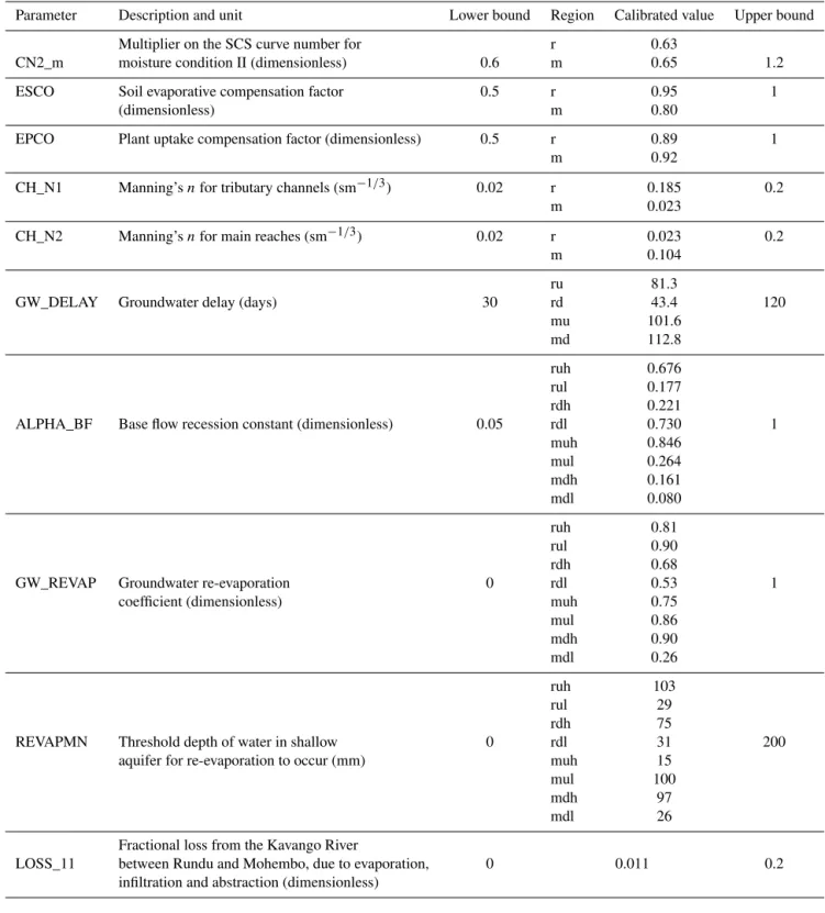
Table 3 provides an overview of the calibration parame-ters and their allowed ranges. For the groundwater param-eters, spatial variation was allowed between the Rundu and Mohembo regions, the upstream and downstream catchments within each region and the high-slope and low-slope portions of the land surface. This resulted in a total number of 19 cal-ibration parameters for the Rundu region and 20 calcal-ibration parameters for the Mohembo region. We chose eight plexes in the SCE calibration run and the number of com-plexes remained the same throughout the run. Both the num-ber of parameter sets in each complex and the numnum-ber of evolution steps before complex shuffling were set to 39 and 41 for the Rundu and Mohembo regions, respectively. The convergence criterion was set to a relative improvement of the best objective function of 1 % over 10 shuffling loops. A total of 50 000 model runs were allowed; however, the cal-ibration converged after 14 711 and 18 373 model runs for the Rundu and Mohembo regions, respectively. After com-pletion of the SCE run, the evolution of the parameter values over the course of the shuffling loops was evaluated. All
pa-rameter values converged to a stable solution away from the a priori parameter bounds.
2.5 Assimilation strategy
The objective of data assimilation is to combine, at each point in time, the model-based estimate of the state of the system as well as the most recent observations of the state, in order to produce the best possible estimate of the current and fu-ture states, taking into account the respective uncertainties of simulated states and observations. The assimilation strategy chosen in this study consists of updating the simulated dis-charge in the Muskingum routing model only, because the objective was to generate probabilistic river discharge fore-casts with lead times of up to 7 days. Updates of the rainfall-runoff model states would probably improve long-term fore-casts significantly but may have limited effect on forefore-casts with short lead times in large basins such as the Kavango Basin. Moreover, updating the rainfall-runoff model would require ensemble-based assimilation approaches. For the in-tended user group of the TIGER-NET products, simplicity and efficiency are key criteria.
Observed in situ discharge at the station Rundu was as-similated to the model in the operational runs. Because the Muskingum routing operator is linear and the measurement operator is linear too, we could use the standard Kalman fil-ter for state updating, since it is the optimal sequential as-similation method for linear dynamics (Kalman, 1960). The Kalman filter simultaneously updates discharge at all basin outlets. If instead of river discharge, water level measure-ments from spaceborne or ground-based instrumeasure-ments are as-similated, the measurement operator becomes non-linear and the extended Kalman filter can be used (Michailovsky et al., 2013). The reader is referred to the literature (e.g., Jazwinski, 1970) for a detailed discussion of the Kalman filter equations and to Michailovsky et al. (2013) for a detailed description of the assimilation approach.
2.6 Description of the model error
Table 3.Model calibration parameters. Subcatchment IDs for the various regions: r=2+3+5+6+7+9+10; m=1+4+8+11+12; ru=2+3; rd=5+6+7+9+10; mu=1; md=4+8+11+12; ruh: HRUs in region ru with terrain slope above 2 %; rul: HRUs in region ru with terrain slope below 2 %; rdh: HRUs in region rd with terrain slope above 2 %; rdl: HRUs in region rd with terrain slope below 2 %; muh: HRUs in region mu with terrain slope above 2 %; mul: HRUs in region mu with terrain slope below 2 %; mdh: HRUs in region md with terrain slope above 2%; mdl: HRUs in region md with terrain slope below 2 %.
Parameter Description and unit Lower bound Region Calibrated value Upper bound Multiplier on the SCS curve number for r 0.63
CN2_m moisture condition II (dimensionless) 0.6 m 0.65 1.2 ESCO Soil evaporative compensation factor 0.5 r 0.95 1
(dimensionless) m 0.80
EPCO Plant uptake compensation factor (dimensionless) 0.5 r 0.89 1
m 0.92
CH_N1 Manning’snfor tributary channels (sm−1/3) 0.02 r 0.185 0.2
m 0.023
CH_N2 Manning’snfor main reaches (sm−1/3) 0.02 r 0.023 0.2
m 0.104 ru 81.3
GW_DELAY Groundwater delay (days) 30 rd 43.4 120 mu 101.6
md 112.8 ruh 0.676 rul 0.177 rdh 0.221
ALPHA_BF Base flow recession constant (dimensionless) 0.05 rdl 0.730 1 muh 0.846
mul 0.264 mdh 0.161 mdl 0.080 ruh 0.81 rul 0.90 rdh 0.68
GW_REVAP Groundwater re-evaporation 0 rdl 0.53 1 coefficient (dimensionless) muh 0.75
mul 0.86 mdh 0.90 mdl 0.26 ruh 103 rul 29 rdh 75
REVAPMN Threshold depth of water in shallow 0 rdl 31 200 aquifer for re-evaporation to occur (mm) muh 15
mul 100 mdh 97 mdl 26 Fractional loss from the Kavango River
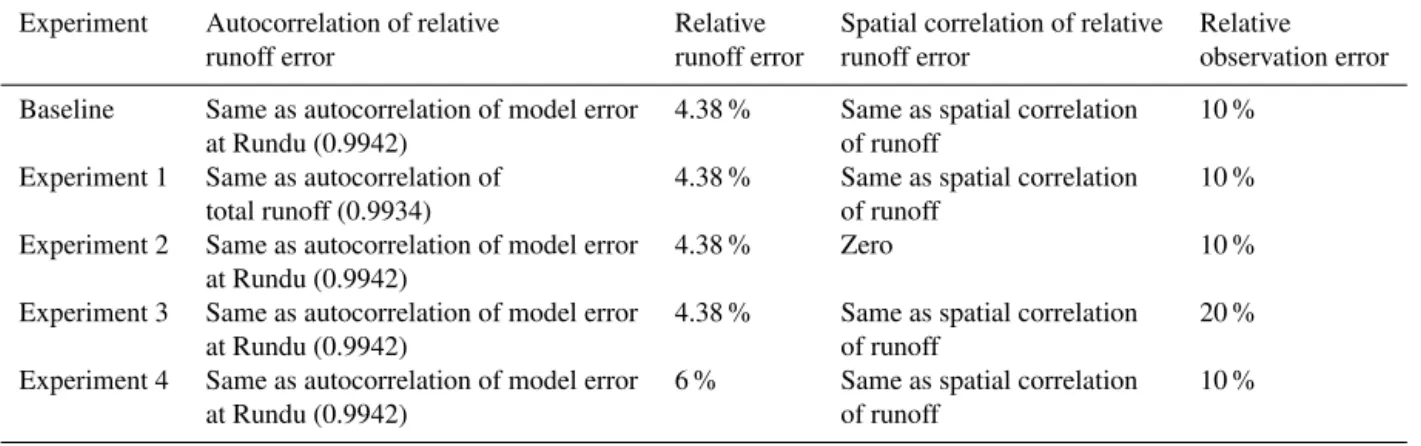
Table 4.Overview of the different forecasting experiments.
Experiment Autocorrelation of relative Relative Spatial correlation of relative Relative runoff error runoff error runoff error observation error Baseline Same as autocorrelation of model error 4.38 % Same as spatial correlation 10 %
at Rundu (0.9942) of runoff
Experiment 1 Same as autocorrelation of 4.38 % Same as spatial correlation 10 % total runoff (0.9934) of runoff
Experiment 2 Same as autocorrelation of model error 4.38 % Zero 10 % at Rundu (0.9942)
Experiment 3 Same as autocorrelation of model error 4.38 % Same as spatial correlation 20 % at Rundu (0.9942) of runoff
Experiment 4 Same as autocorrelation of model error 6 % Same as spatial correlation 10 % at Rundu (0.9942) of runoff
residuals at the available in situ discharge stations:
wt =
Qsim,t−Qobs,t Qobs,t
, (3)
wherewtis the relative model residual (–),Qsim,tis the mod-eled discharge at the in situ discharge station at time stept
andQobs,t is the in situ discharge as time stept. The auto-correlation of the residuals was assumed to be represented by a first-order autoregressive (AR1) model:
wt =δwt−1+εt, (4)
whereδis the AR1 parameter andεis a sequence of white Gaussian noise with a spatial covarianceQ′. Due to the
cor-related meteorological inputs the runoff forcing error was assumed to be spatially correlated between the various sub-catchments of the model. In the baseline experiment, we as-sume that the spatial correlation of the runoff forcing error is equivalent to the spatial correlation of the runoff forcing itself. The correlation matrix of the runoff inputs was com-puted andQ′was set to
Q′=Cσ (ǫ)2, (5)
where C is the runoff correlation matrix and σ (ǫ)2 is the variance of the white noise component of the AR1 model. The auto-correlated runoff error state was integrated in the Kalman filter updating scheme by augmenting the model state vector with the correlated noise term (Jazwinski, 1970; Michailovsky et al., 2013). This ensures persistence of as-similation benefits in time.
The major source of error in in situ discharge observations is the rating curve, which is used to transform readings of river stage into river discharge. Rating curves are particularly unreliable for extreme flow rates and, depending on the chan-nel characteristics, the rating curve changes over time and requires frequent updating. In the absence of detailed infor-mation on the in situ measurement procedure, we assumed the measurement error to be uncorrelated in time and propor-tional to the discharge. In the baseline experiment, the rela-tive error was assumed to be 10 %, which is a typical value
for in situ discharge derived from rating curves (Di Baldas-sarre and Montanari, 2009) and comparable to other hydro-logic data assimilation studies (e.g., Clark et al., 2008; Geor-gakakos, 1986; Weerts and El Serafy, 2006).
In order to evaluate the impact of model error and obser-vation error specifications on the performance of the prob-abilistic discharge forecasts, four additional forecasting ex-periments were conducted. Table 4 presents an overview of the experiments. In the baseline experiment, the autocorre-lation of the relative runoff error was set equal to the auto-correlation of the relative model error at Rundu (0.9942), as described above. The magnitude of the relative runoff error was set to 4.38 %, which is the same as the relative model er-ror at Rundu. The spatial correlation of relative runoff erer-ror was set equal to the spatial correlation of runoff and the rel-ative observation error was set to 10 %. In experiment 1, the autocorrelation of the runoff error was set equal to the auto-correlation of the spatially aggregated runoff (0.9934) while the other specifications are the same as in the baseline run. In experiment 2, the spatial correlation of the runoff error was set to zero and all other specifications are as in the baseline run. In experiment 3, the runoff error specifications are the same as in the baseline and the relative observation error was set to 20 %. Finally, in experiment 4, the white noise compo-nent of the relative runoff error was increased from 4.38 to 6 % and all other specifications are as in the baseline run.
2.7 Operational forecasting and performance evaluation
follow-ing criteria were used to assess the performance of the cen-tral model forecast: Nash–Sutcliffe model efficiency (NSE), root-mean-square error (RMSE), mean error (ME) and per-sistence index (PI). The PI (Bennett et al., 2013) is defined analogous to the NSE:
PI= 1 n
n P
i=1
Qi−Qobs,i 2
−1n n P
i=1
(Qi−Qlast)2
−1n n P
i=1
(Qi−Qlast)2
, (6)
where n is the number of forecasted observations, Q are the forecasts,Qobsare the observations andQlastis the lat-est available observation before the forecasted observation. While the NSE uses the average of the observations as the benchmark (i.e., a forecast that performs as good as the long-term average of the available observations scores an NSE of 0), the PI uses the last available observation as the benchmark (i.e., a forecast that performs as good as the latest available observation scores a PI of 0).
Reliability and sharpness of the probabilistic forecasts were assessed with the coverage of the 95 % confidence inter-val (i.e., percentage of observations that fall within the pre-dicted nominal 95 % confidence interval), the sharpness of the 95 % confidence interval (width of predicted 95 % con-fidence interval), the interval skill score (ISS) of the 95 % confidence interval and the continuous ranked probability score (CRPS). The ISS is defined according to Gneiting and Raftery (2007) as
ISSα= n X
i=1
issα li, ui, Qobs,i,
issα(l, u, Qobs)=
( (u
−l) if l < Qobs< u
(u−l)+2/α(l−x) if Qobs< l
(u−l)+2/α(x−u) if Qobs> u
, (7)
whereαis the level of the confidence interval (0.05 in our case),lis the lower anduthe upper bound of the confidence interval.
The CRPS is a verification tool for probabilistic forecasts and can be interpreted as the area between the cumulative distribution function of the forecast and the cumulative dis-tribution function of the observation, which is a Heaviside step function. The CRPS thus compares the full distribution function of the forecast with the observation and not only selected confidence intervals. For normally distributed fore-casts, a closed-form expression for the CRPS exists (Gneiting et al., 2004):
CRPS=n1 n X
i=1
crps Qobs,i, Qi, σi, (8)
crps(Qobs, Q, σ )=σ Q
obs−Q
σ
28
Q
obs−Q
σ
−1
+2φ
Q
obs−Q
σ
−√1π
,
whereσ is the standard deviation of the probabilistic fore-cast,8is the cumulative distribution function andφthe prob-ability density function of the standard normal distribution. For a deterministic forecast, the CRPS is equivalent to the mean absolute error (Boucher et al., 2011; Schellekens et al., 2011). This allows for a systematic and objective comparison between deterministic and probabilistic forecasts.
The performance of operational forecasts was compared to two benchmark forecasts which can be produced with mini-mal effort: persistence and climatology. Persistence forecasts the flow as equal to the last available observation, while cli-matology forecasts the flow as equal to the historical average flow for this day of the year.
3 Results
3.1 Comparison of precipitation products
system is continuously updated and modified (process pa-rameterization, spatial resolution, etc.), performance of pre-cipitation forecasts should be regularly checked during op-erational application of the hydrologic forecasting system. Changes in the quantitative precipitation forecasts may re-quire adjustments in the bias correction and/or recalibration of the hydrological model.
Clearly, the quality of the precipitation forcing is a critical issue which has significant control over the performance of the forecasting system. Within the TIGER-NET framework, we are dependent on public domain data sets and NOAA-GFS was the only free source of operational weather fore-casts for the African continent available to the project. Po-tentially, model performance could be improved if NOAA-GFS data was corrected dynamically, for instance, by con-tinuously benchmarking it against real-time or near real-time precipitation products such as FEWS-RFE or TRMM-3B42 (Huffman et al., 2007) for the recent past and estimating a time-variable bias correction. An even better solution would be to merge NOAA-GFS data with in situ precipitation data. However, no operational data set of in situ precipitation ob-servations is available for this part of Africa.
3.2 Performance of the calibrated model
Table 3 provides an overview of the calibrated parameter values. All parameter values are physically reasonable and calibrated parameter values do not stick to the bounds of a-priori parameter intervals. Figures 3 and 4 show model per-formance in the calibration and validation periods.
Model residuals were analyzed and tested for normality and autocorrelation. Figure 5 summarizes the results of the model error analysis for the station Rundu. Figure 5a plots the relative error of the hydrologic–hydrodynamic model ver-sus the observed discharge. Obviously, the relative error is not independent of discharge; it is higher for low discharge than for high discharge. The Q–Q (quantile–quantile) plot in Fig. 5b shows that the empirical distribution of model errors significantly deviates from a normal distribution. The empir-ical distribution of the model errors is narrower than the nor-mal distribution and a larger portion of the data are clustered around the mean. The correlogram in Fig. 5c shows highly significant auto-correlation of the model errors. Figure 5d shows the residual model errors (ε) after application of the AR1 model (Eq. 4), plotted against the observed discharge. This distribution looks more even than the distribution of the primary model residuals in Fig. 5a. A test for normality us-ing the Q–Q plot shows significant deviations and again a narrower distribution than the normal distribution (Fig. 5e). Temporal correlations have been effectively removed from the model errors and no significant correlations remain as shown in Fig. 5f. We conclude from this analysis that the relative error of the hydrologic–hydrodynamic model can be reasonably represented with an AR1 model. The time corre-lation of the AR1 model isδ=0.9942 on the daily time step.
The random error contribution isε=0.0438. As explained in the methods section, we assume, in the baseline experi-ment, that the same AR1 model parameters can represent the relative error of the runoff forcing and we use this result to parameterize the model error in the Kalman filter assimila-tion scheme.
3.3 Discharge forecasting and data assimilation
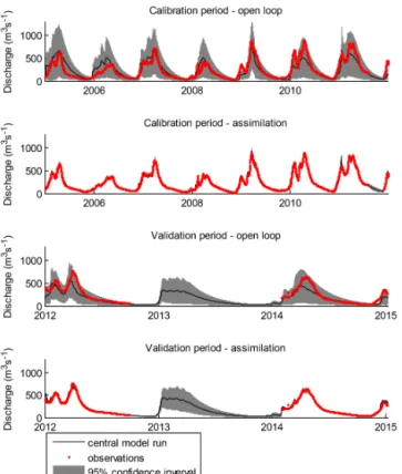
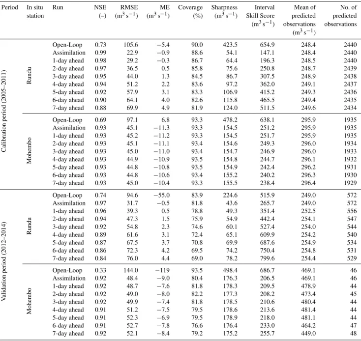
Table 5 reports the performance statistics for the probabilistic model runs. We report results for the open-loop run without assimilation, the assimilation run (“nowcasting”) as well as the 1–7-day ahead forecasts. The various forecasting hori-zons use different precipitation forcings (forecasts available at the simulated issue date) and in situ data are assimilated up to simulated issue date. We only assimilate data from the station Rundu because (i) no real-time observations are avail-able for Mohembo and (ii) this enavail-ables us to assess the effect of upstream assimilation on a downstream station. The indi-cators are reported for both in situ stations and for the cali-bration and the validation periods. We are well aware that the observations in the calibration period have been used already for model calibration and are now used again for assimila-tion. Still, we feel that it is useful to present the statistics for information. Figure 6 shows the open-loop and assimilation run for the station Rundu during calibration and validation periods. We first assess the performance of the probabilistic open-loop run. Generally, the chosen error model seems to be appropriate. The forecasts produced by the open-loop run are reliable; the coverage of the nominal 95 % confidence in-terval does not fall below 84 % at any of the stations during any of the periods. However, the open-loop forecasts are not very sharp, as evidenced by the wide confidence intervals in Fig. 6. This results in a relatively high ISS score.
Figure 2.Left: double mass plot of the FEWS-RFE and NOAA-GFS precipitation products averaged over the entire Kavango River basin. Right: double mass plots of the 1-day ahead forecasted NOAA-GFS precipitation and the 2–7-day ahead forecasted NOAA-GFS precipitation averaged over the entire Kavango River basin.
Figure 3.Observed (red dots) and simulated (black lines) hydro-graphs for the calibration period for Rundu (top) and Mohembo (bottom).
is over-compensated by loss of reliability, which leads to in-creasing ISS scores with inin-creasing lead time. For the valida-tion period, only the 0–3 ahead forecasts are better than the open-loop run, if evaluated with the ISS score.
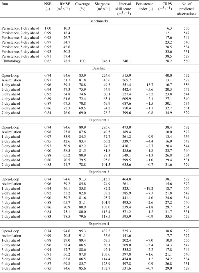
Table 6 summarizes the performance of the operational forecasts produced in the different forecasting experiments for the validation period and the station Rundu. Results are reported for the baseline and experiments 1, 3 and 4. Exper-iment 2 produced results that are very similar to the baseline results and those are therefore not separately reported. Ta-ble 6 also includes the performance indicators for the persis-tence and climatology benchmarks.
Experiment 4 generally shows the best performance. Ac-cording to the CRPS score, the forecasts are superior to the open-loop run for all forecasting horizons. Forecasts are also better than the persistence benchmarks for forecasting
hori-Figure 4.Observed (red dots) and simulated (black lines) hydro-graphs for the validation period for Rundu (top) and Mohembo (bot-tom).
zons between 4 and 7 days. For forecasting horizons be-tween 1 and 6 days, the model outperforms the climatology benchmark. The persistence index indicates that the forecast-ing system performs worse than the persistence benchmark. However, it is important to note that the PI does not assess the quality of probabilistic forecasts in terms of sharpness and reliability but only takes the central forecast into account and compares two deterministic predictions.
Figure 5. (a) Relative error of the hydrologic–hydrodynamic model vs. observed discharge.(b) Q–Q plot of the relative errors shown in(a).(c)Correlogram of the relative errors shown in(a).(d)Relative errors of hydrologic–hydrodynamic model after removal of the time-correlated part plotted vs. observed discharge.(e)Q–Q plot of the relative errors shown in(d).(f)Correlogram of the relative errors shown in(d).
Figure 6.Probabilistic simulation of river discharge in the open-loop and assimilated run for the calibration and the validation peri-ods for the station Rundu.
4 Discussion
The presented approach for the generation of probabilistic river discharge forecasts is simple and robust and designed to work in data-sparse and poorly gauged basins. A key fac-tor for the performance of the system is the rainfall forcing. While the NOAA-GFS rainfall can produce reasonably reli-able and sharp forecasts for the Kavango River, the product should be further compared against other operational precip-itation products. Promising avenues for future research may be dynamic bias correction using other precipitation or soil moisture products and/or the extension of the forecast lead time beyond 7 days. NOAA-GFS does provide forecasts up to 16 days into the future. However, the spatial resolution is reduced by a factor of 2 for forecasting horizons beyond 1 week. To further improve the reliability and sharpness of the forecasts, an ensemble of weather forecasts should be used to drive the forecasting system (Cloke and Pappen-berger, 2009). One potential source of free ensemble weather forecasts for the African continent is the Global Ensemble Forecasting System (GEFS; http://www.emc.ncep.noaa.gov/ ?branch=GEFS).
pa-Table 5.Performance of the operational model in the calibration and validation periods.
Period In situ Run NSE RMSE ME Coverage Sharpness Interval Mean of No. of
station (–) (m3s−1) (m3s−1) (%) (m3s−1) Skill Score predicted predicted
(m3s−1) observations observations
(m3s−1)
Calibration
period
(2005–2011)
Rundu
Open-Loop 0.73 105.6 −5.4 90.0 423.5 654.9 248.4 2440
Assimilation 0.99 22.9 −0.9 88.6 54.1 147.1 248.4 2440
1-day ahead 0.98 29.2 −0.3 86.7 64.4 196.3 248.5 2440
2-day ahead 0.97 36.5 0.5 85.8 75.6 250.8 248.7 2439
3-day ahead 0.95 44.0 1.3 84.5 86.7 307.5 248.9 2438
4-day ahead 0.94 51.2 2.2 83.6 97.2 362.0 249.1 2437
5-day ahead 0.92 57.9 3.1 83.3 106.9 415.2 249.3 2436
6-day ahead 0.90 64.1 4.0 82.6 115.8 465.5 249.4 2435
7-day ahead 0.88 69.9 4.9 81.9 124.0 511.5 249.6 2434
Mohembo
Open-Loop 0.69 97.1 6.8 93.3 478.2 638.1 295.9 1935
Assimilation 0.93 45.1 −11.3 93.3 154.5 251.2 295.9 1935
1-day ahead 0.93 45.2 −11.2 93.3 154.5 251.7 295.9 1935
2-day ahead 0.93 45.1 −11.1 93.4 154.6 249.3 296.0 1934
3-day ahead 0.93 45.0 −11.0 93.4 154.7 246.9 296.0 1933
4-day ahead 0.93 44.9 −10.9 93.5 154.8 244.7 296.1 1932
5-day ahead 0.93 44.8 −10.8 93.5 154.9 242.4 296.2 1931
6-day ahead 0.93 44.8 −10.6 93.4 155.2 240.2 296.3 1930
7-day ahead 0.93 45.0 −10.4 93.3 155.5 238.4 296.4 1929
V
alidation
period
(2012–2014)
Rundu
Open-Loop 0.74 94.6 −55.0 83.9 224.6 515.9 249.0 572
Assimilation 0.97 31.7 −0.5 81.8 43.6 265.7 249.0 572
1-day ahead 0.96 39.3 0.5 78.8 49.3 351.4 252.5 556
2-day ahead 0.94 47.3 1.5 75.9 54.9 442.4 254.1 547
3-day ahead 0.92 54.8 2.3 74.6 60.1 527.4 254.0 544
4-day ahead 0.89 61.6 3.1 72.4 65.1 609.9 254.2 540
5-day ahead 0.87 67.5 3.7 70.8 69.9 687.6 254.9 534
6-day ahead 0.86 72.3 4.2 69.5 74.2 750.4 254.8 531
7-day ahead 0.84 76.0 4.4 69.0 78.2 799.6 254.4 529
Mohembo
Open-Loop 0.33 144.0 −119 93.5 498.4 686.7 469.1 46
Assimilation 0.92 48.4 −9.0 80.4 176.3 206.5 469.1 46
1-day ahead 0.92 48.7 −7.6 81.8 178.3 209.5 478.9 44
2-day ahead 0.92 49.0 −8.0 82.2 177.3 208.2 473.4 45
3-day ahead 0.92 49.9 −7.4 81.8 178.5 210.6 480.4 44
4-day ahead 0.91 51.2 −7.5 79.5 178.6 213.6 481.4 44
5-day ahead 0.91 52.3 −6.9 79.5 178.9 218.0 481.1 44
6-day ahead 0.91 52.7 −7.8 76.6 176.4 233.0 464.2 47
7-day ahead 0.92 52.1 −8.4 79.2 175.2 255.7 449.0 48
rameters of the routing model, because we assume that these error contributions are minor compared to the runoff error. While this approach is robust and efficient, it clearly rep-resents a strong simplification of reality. It is clear that the simple Muskingum routing model has significant structural error, for instance due to the fact that floodplains and surface water/groundwater interactions are not simulated.
Comparison of the various forecasting experiments shows that assumptions about the model and observation errors have a large impact on the performance of the forecasting system. The magnitude of the relative runoff error is particularly sen-sitive, as evidenced by the improved performance of experi-ment 4 compared to the baseline. It is reasonable to assume
Table 6.Performance indicators for the forecasts issued for the station Rundu in the validation period, excluding model “warm-up” periods.
Run NSE RMSE Coverage Sharpness Interval Persistence CRPS No. of
(–) (m3s−1) (%) (m3s−1) skill score index (–) (m3s−1) predicted
(m3s−1) observations
Benchmarks
Persistence, 1-day ahead 1.00 10.3 6.3 556
Persistence, 2-day ahead 0.99 18.4 12.1 547
Persistence, 3-day ahead 0.98 26.7 17.6 544
Persistence, 4-day ahead 0.97 34.7 23.2 540
Persistence, 5-day ahead 0.95 42.6 28.5 534
Persistence, 6-day ahead 0.93 50.2 33.6 531
Persistence, 7-day ahead 0.91 57.4 38.5 529
Climatology 0.82 78.5 100 346.1 346.1 28.2 580
Baseline
Open-Loop 0.74 94.6 83.9 224.6 515.9 40.0 572
Assimilation 0.97 31.7 81.8 43.6 265.7 13.1 572
1-day ahead 0.96 39.3 78.8 49.3 351.4 −13.7 16.7 556
2-day ahead 0.94 47.3 75.9 54.9 442.4 −5.6 20.3 547
3-day ahead 0.92 54.8 74.6 60.1 527.4 −3.2 23.8 544
4-day ahead 0.89 61.6 72.4 65.1 609.9 −2.1 27.1 540
5-day ahead 0.87 67.5 70.8 69.9 687.6 −1.5 30.1 534
6-day ahead 0.86 72.3 69.5 74.2 750.4 −1.1 32.7 531
7-day ahead 0.84 76.0 69.0 78.2 799.6 −0.8 34.9 529
Experiment 1
Open-Loop 0.74 94.6 89.9 295.6 473.0 38.4 572
Assimilation 0.98 25.8 87.6 49.5 189.4 10.0 572
1-day ahead 0.97 33.9 84.5 57.7 261.2 −9.9 13.4 556
2-day ahead 0.95 42.6 83.4 66.2 339.7 −4.4 16.9 547
3-day ahead 0.93 50.9 82.2 74.2 416.1 −2.7 20.4 544
4-day ahead 0.90 58.5 81.5 81.8 485.6 −1.8 23.7 540
5-day ahead 0.88 65.2 80.9 89.1 549.1 −1.3 26.8 534
6-day ahead 0.86 70.5 79.5 95.6 599.5 −1.0 29.4 531
7-day ahead 0.85 74.7 78.8 101.5 635.6 −0.7 31.6 529
Experiment 3
Open-Loop 0.74 94.6 91.3 315.5 464.8 38.1 572
Assimilation 0.96 39.2 85.8 74.9 261.1 15.6 572
1-day ahead 0.94 46.1 83.8 82.2 323.1 −19.2 18.7 556
2-day ahead 0.92 53.2 82.8 89.2 385.9 −7.3 21.8 547
3-day ahead 0.90 59.7 81.6 95.7 441.1 −4.0 24.6 544
4-day ahead 0.88 65.7 81.1 101.9 493.5 −2.6 27.2 540
5-day ahead 0.86 70.9 80.9 108.0 539.4 −1.8 29.7 534
6-day ahead 0.84 75.1 80.0 113.4 571.2 −1.2 31.7 531
7-day ahead 0.83 78.5 79.6 118.5 595.9 −0.9 33.3 529
Experiment 4
Open-Loop 0.74 94.6 95.3 432.2 525.3 38.6 572
Assimilation 0.99 20.5 91.1 55.6 141.6 7.7 572
1-day ahead 0.98 29.0 89.4 67.5 202.4 −7.0 10.8 556
2-day ahead 0.96 38.4 88.5 80.1 269.0 −3.4 14.3 547
3-day ahead 0.94 47.7 88.6 92.1 335.2 −2.2 17.8 544
4-day ahead 0.91 56.2 87.8 103.6 397.8 −1.6 21.1 540
5-day ahead 0.89 63.8 86.5 114.4 454.0 −1.2 24.2 534
6-day ahead 0.87 69.8 85.7 123.9 497.8 −0.9 26.8 531
Figure 7.Performance of the 0–7-day ahead probabilistic forecasts in the validation period at Rundu station for experiment 4. The black solid line is the central forecast. Grey shading indicates the 95 % confidence interval of the forecast and red dots are observations. Blue bars indicate daily forecasted precipitation from NOAA-GFS.
Figure 8.Predictive Q–Q plots for the station Rundu and the validation period for experiment 4.
close to the baseline, because the spatial correlation of runoff between the different subcatchments is low, due to the vari-able hydrologic characteristics of the subcatchments. Predic-tive Q–Q plots for experiment 4 (Fig. 8) indicate significant deviations of the empirical distribution of normalized fore-cast errors from the normal distribution.
As is common for studies dealing with probabilistic river discharge forecasting, we find that our probabilistic forecasts
We generally observe weaker performance of the forecast-ing system in the beginnforecast-ing of the rainy season, i.e., after the long dry season during the onset of the annual high-flow season. This may be due to deficiencies in the precipitation forecasts and/or due to weaknesses in the representation of hydrological processes in the SWAT model. It appears that, in reality, the first rains in the early rainy season already lead to increased river flow, while in the model these precipita-tion events are completely absorbed in the various simulated hydrological storage compartments.
In this study, focus has been on the final output of the mod-eling chain, i.e., river discharge. However, SWAT simulates a multitude of intermediate states and fluxes in the land phase of the hydrological cycle, which could be analyzed and com-pared to observations, if such observations were available. There is an obvious opportunity to inform the modeling sys-tem with other types of in situ and remote sensing obser-vations such as radar altimetry, soil moisture and total wa-ter storage from time-variable gravity (Milzow et al., 2011). However, if such data were to be formally assimilated to the modeling system, an ensemble approach would have to be chosen because of the highly non-linear responses inherent in the SWAT model. Many studies have addressed ensemble-based streamflow forecasting with lumped-conceptual or dis-tributed hydrological models. Rakovec et al. (2012) found that rainfall-runoff model states were less sensitive compared to routing states in their hydrologic data assimilation study with the ensemble Kalman filter and suggested time lags between the rainfall-runoff model states and streamflow re-sponse as the likely reason. Alternative updating strategies that use several previous time steps instead of the last time step only (e.g., Ensemble Kalman Smoother) can potentially solve these problems. Other recurring issues in such studies are high computational demand and model error parameteri-zation (e.g., Clark et al., 2008).
5 Conclusions
We have presented an operational probabilistic river dis-charge forecasting system for poorly gauged basins which re-lies exclusively on public-domain, open-source software and data. The forecasting system is specifically adapted to the conditions prevailing in many African basins, such as weak in situ monitoring infrastructure, budget constraints for op-erational monitoring and management as well as weak insti-tutional capacity. We demonstrated the performance of the forecasting system for the Kavango River and obtained en-couraging results. The 0–7-day ahead probabilistic forecasts produced by the system are sharp and reliable. The system may benefit from ingestion of other types of in situ or re-motely sensed observations such as radar altimetry and soil moisture. The TIGER-NET project and its Water Observa-tion and InformaObserva-tion System (WOIS) provide an ideal plat-form to combine remote sensing observations and
hydrolog-ical models to generate accurate estimates of hydrologhydrolog-ical states as well as sharp and reliable forecasts for operational water resources management.
Acknowledgements. We acknowledge funding from the European Space Agency (ESA) through the TIGER-NET project. Real-time and historical in situ observations for the station Rundu were provided by Namibia’s Ministry of Agriculture Water and Forestry. Historical in situ observations for the station Mohembo were provided by Botswana’s Department of Water Affairs.
Edited by: E. Toth
References
Arnold, J. G., Moriasi, D. N., Gassman, P. W., Abbaspour, K. C., White, M. J., Srinivasan, R., Santhi, C., Harmel, R. D., van Griensven, A., Van Liew, M. W., Kannan, N., and Jha, M. K.: SWAT: model use, calibration, and validation, Trans. ASABE, 55, 1491–1508, 2012.
Bennett, N. D., Croke, B. F. W., Guariso, G., Guillaume, J. H. A., Hamilton, S. H., Jakeman, A. J., Marsili-Libelli, S., Newham, L. T. H., Norton, J. P., Perrin, C., Pierce, S. A., Robson, B., Sep-pelt, R., Voinov, A. A., Fath, B. D., and Andreassian, V.: Charac-terising performance of environmental models, Environ. Model. Softw., 40, 1–20, doi:10.1016/j.envsoft.2012.09.011, 2013. Berry, P. A. M., Smith, R. G., and Benveniste, J.: ACE2: The New
Global Digital Elevation Model, in: Gravity, Geoid And Earth Observation, edited by: Mertikas, S. P., International Association of Geodesy Symposia, Crete, Greece, 23–27 June 2008, 231– 237, doi:10.1007/978-3-642-10634-7_30, 2010.
Biancamaria, S., Durand, M., Andreadis, K. M., Bates, P. D., Boone, A., Mognard, N. M., Rodríguez, E., Alsdorf, D. E., Lettenmaier, D. P., and Clark, E. A.: Assimilation of virtual wide swath al-timetry to improve Arctic river modeling, Remote Sens. Envi-ron., 115, 373–381, doi:10.1016/j.rse.2010.09.008, 2011. Boucher, M.-A., Anctil, F., Perreault, L., and Tremblay, D.: A
comparison between ensemble and deterministic hydrological forecasts in an operational context, Adv. Geosci., 29, 85–94, doi:10.5194/adgeo-29-85-2011, 2011.
Chow, V. T., Maidment, D. R., and Mays, L. W.: Applied Hydrol-ogy, Water Resources and Environmental Engineering, McGraw-Hill, New York, 1988.
Clark, M. P., Rupp, D. E., Woods, R. A., Zheng, X., Ibbitt, R. P., Slater, A. G., Schmidt, J., and Uddstrom, M. J.: Hy-drological data assimilation with the ensemble Kalman fil-ter: Use of streamflow observations to update states in a dis-tributed hydrological model, Adv. Water Resour., 31, 1309– 1324, doi:10.1016/j.advwatres.2008.06.005, 2008.
Cloke, H. L. and Pappenberger, F.: Ensemble flood forecasting: A review, J. Hydrol., 375, 613–626, doi:10.1016/j.jhydrol.2009.06.005, 2009.
Di Baldassarre, G. and Montanari, A.: Uncertainty in river discharge observations: a quantitative analysis, Hydrol. Earth Syst. Sci., 13, 913–921, doi:10.5194/hess-13-913-2009, 2009.
anal-ysis, available at: http://www.pesthomepage.org/Home.php, last access: 16 July, 2014.
Duan, Q. Y., Sorooshian, S., and Gupta, V.: Effective and efficient global optimization for conceptual rainfall-runoff models, Water Resour. Res., 28, 1015–1031, doi:10.1029/91WR02985, 1992. FAO-UNESCO: Soil map of the world 1:5 000 000, Paris, France,
1974.
Fekete, B. M. and Voeroesmarty, C. J.: The current status of global river discharge monitoring and potential new technologies com-plementing traditional discharge measurements, in: Proceedings of the PUB Kick-off Meeting, Brasilia, Brazil, 20–22 November 2002, IAHS Publication 309, 2007.
Folwell, S. and Farqhuarson, F.: The impacts of climate change on water resources in the Okavango basin, in: Climate Variability and Change – Hydrological Impacts, edited by: Demuth, S., Gus-tard, A., Planos, E., Scatena, F., and Servat, E., IAHS publication, 382–388, 2006.
Gassman, P. W., Reyes, M. R., Green, C. H., and Arnold, J. G.: SWAT Peer-Reviewed Literature: A Review, Hydrol. Process., 13, 1–17, 2005.
Georgakakos, K. P.: A generalized stochastic hydrometeo-rological model for flood and flash-flood forecasting – Part 2: case studies, Water Resour. Res., 22, 2096–2106, doi:10.1029/WR022i013p02096, 1986.
George, C. and Leon, L. F.: WaterBase?: SWAT in an open source GIS, Open Hydrol. J., 1, 19–24, 2007.
Gneiting, T. and Raftery, A. E.: Strictly proper scoring rules, pre-diction, and estimation, J. Am. Stat. Assoc., 102, 359–378, doi:10.1198/016214506000001437, 2007.
Gneiting, T., Westveld, A. H., Raftery, A. E., and Goldman, T.: Cal-ibrated Probabilistic Forecasting Using Ensemble Model Output Statistics and Minimum CRPS Estimation, Seattle, Washington, USA, 2004.
Guzinski, R., Kass, S., Huber, S., Bauer-Gottwein, P., Jensen, I. H., Naeimi, V., Doubkova, M., Walli, A., and Tottrup, C.: A Wa-ter Observation and Information System for Integrated WaWa-ter Resource Management in Africa, Remote Sens., 6, 7819–7839, doi:10.3390/rs6087819, 2014.
Herman, A., Kumar, V. B., Arkin, P. A., and Kousky, J. V.: Objec-tively determined 10-day African rainfall estimates created for famine early warning systems, Int. J. Remote Sens., 18, 2147– 2159, doi:10.1080/014311697217800, 1979.
Huffman, G. J., Bolvin, D. T., Nelkin, E. J., Wolff, D. B., Adler, R. F., Gu, G., Hong, Y., Bowman, K. P., and Stocker, E. F.: The TRMM Multisatellite Precipitation Analy-sis (TMPA): Quasi-Global, Multiyear, Combined-Sensor Precip-itation Estimates at Fine Scales, J. Hydrometeorol., 8, 38–55, doi:10.1175/JHM560.1, 2007.
Hughes, D. A., Andersson, L., Wilk, J., and Savenije, H. H. G.: Re-gional calibration of the Pitman model for the Okavango River, J. Hydrol., 331, 30–42, doi:10.1016/j.jhydrol.2006.04.047, 2006. Hughes, D. A., Kingston, D. G., and Todd, M. C.: Uncertainty in
water resources availability in the Okavango River basin as a re-sult of climate change, Hydrol. Earth Syst. Sci., 15, 931–941, doi:10.5194/hess-15-931-2011, 2011.
Jazwinski, A. H.: Stochastic Processes and Filtering Theory, Aca-demic Press, New York, USA, 1970.
Kalman, R. E.: A New Approach to Linear Filtering and Prediction Problems, J. Basic Eng., 82, 35–45, 1960.
Kgathi, D. L., Kniveton, D., Ringrose, S., Turton, A. R., Vanderpost, C. H. M., Lundqvist, J., and Seely, M.: The Okavango; a river supporting its people, environment and economic development, J. Hydrol., 331, 3–17, doi:10.1016/j.jhydrol.2006.04.048, 2006. Liu, Y., Weerts, A. H., Clark, M., Hendricks Franssen, H.-J., Kumar,
S., Moradkhani, H., Seo, D.-J., Schwanenberg, D., Smith, P., van Dijk, A. I. J. M., van Velzen, N., He, M., Lee, H., Noh, S. J., Rakovec, O., and Restrepo, P.: Advancing data assimilation in operational hydrologic forecasting: progresses, challenges, and emerging opportunities, Hydrol. Earth Syst. Sci., 16, 3863–3887, doi:10.5194/hess-16-3863-2012, 2012.
Madsen, H. and Skotner, C.: Adaptive state updating in real-time river flow forecasting – a combined filtering and error forecasting procedure, J. Hydrol., 308, 302–312, doi:10.1016/j.jhydrol.2004.10.030, 2005.
Maier, H. R., Jain, A., Dandy, G. C., Sudheer, K. P.: Methods used for the development of neural networks for the predic-tion of water resource variables in river systems: Current sta-tus and future directions, Environ. Model. Softw., 25, 891–909, doi:10.1016/j.envsoft.2010.02.003, 2010.
McCarthy, T. S., Cooper, G. R. J., Tyson, P. D., and Ellery, W. N.: Seasonal flooding in the Okavango Delta, Botswana – recent his-tory and future prospects, S. Afr. J. Sci., 96, 25–33, 2000. Michailovsky, C. I., Milzow, C., and Bauer-Gottwein, P.:
As-similation of radar altimetry to a routing model of the Brahmaputra River, Water Resour. Res., 49, 4807–4816, doi:10.1002/wrcr.20345, 2013.
Milzow, C., Kgotlhang, L., Bauer-Gottwein, P., Meier, P., and Kinzelbach, W.: Regional review: the hydrology of the Okavango Delta, Botswana – processes, data and modelling, Hydrogeol. J., 17, 1297–1328, doi:10.1007/s10040-009-0436-0, 2009. Milzow, C., Krogh, P. E., and Bauer-Gottwein, P.: Combining
satel-lite radar altimetry, SAR surface soil moisture and GRACE to-tal storage changes for hydrological model calibration in a large poorly gauged catchment, Hydrol. Earth Syst. Sci., 15, 1729– 1743, doi:10.5194/hess-15-1729-2011, 2011.
Moradkhani, H., Hsu, K.-L., Gupta, H., and Sorooshian, S.: Uncer-tainty assessment of hydrologic model states and parameters: Se-quential data assimilation using the particle filter, Water Resour. Res., 41, W05012, doi:10.1029/2004WR003604, 2005. Nash, J. E. and Sutcliffe, J. V.: River flow forecasting through
con-ceptual models – Part I: a discussion of principles, J. Hydrol., 10, 282–290, 1970.
Neal, J., Schumann, G., Bates, P., Buytaert, W., Matgen, P., and Pappenberger, F.: A data assimilation approach to dis-charge estimation from space, Hydrol. Process., 23, 3641–3649, doi:10.1002/hyp.7518 2009.
Neitsch, S. L., Arnold, J. G., Kiniry, J. R., and Williams, J. R.: Soil & Water Assessment Tool, Theoretical Documentation Version 2009, 2011.
NOAA: GFS Global Forecast System, available at: http://www. emc.ncep.noaa.gov/index.php?branch=GFS, last access: 16 July, 2014.
Pauwels, V. R. N. and De Lannoy, G. J. M.: Ensemble-based assim-ilation of discharge into rainfall-runoff models: A comparison of approaches to mapping observational information to state space, Water Resour. Res., 45, W08428, doi:10.1029/2008WR007590, 2009.
Peterson, T. C. and Vose, R. S.: An overview of the global historical climatology network temperature database, B. Am. Meteorol. Soc., 78, 2837–2849, doi:10.1175/1520-0477(1997)078<2837:AOOTGH>2.0.CO;2, 1997.
Rakovec, O., Weerts, A. H., Hazenberg, P., Torfs, P. J. J. F., and Uijlenhoet, R.: State updating of a distributed hydrological model with Ensemble Kalman Filtering: effects of updating fre-quency and observation network density on forecast accuracy, Hydrol. Earth Syst. Sci., 16, 3435–3449, doi:10.5194/hess-16-3435-2012, 2012.
Schellekens, J., Weerts, A. H., Moore, R. J., Pierce, C. E., and Hildon, S.: The use of MOGREPS ensemble rainfall forecasts in operational flood forecasting systems across England and Wales, Adv. Geosci., 29, 77–84, doi:10.5194/adgeo-29-77-2011, 2011. Seo, D.-J., Koren, V., and Cajina, N.: Real-Time Variational
Assim-ilation of Hydrologic and Hydrometeorological Data into Oper-ational Hydrologic Forecasting, J. Hydrometeorol., 4, 627–641, 2003.
Seo, D.-J., Cajina, L., Corby, R., and Howieson, T.: Auto-matic state updating for operational streamflow forecasting via variational data assimilation, J. Hydrol., 367, 255–275, doi:10.1016/j.jhydrol.2009.01.019, 2009.
Stisen, S. and Sandholt, I.: Evaluation of remote-sensing-based rainfall products through predictive capability in hy-drological runoff modelling, Hydrol. Process., 24, 879–891, doi:10.1002/hyp.7529, 2010.
Tang, Q., Gao, H., Lu, H., Lettenmaier, D. P.: Remote sensing: hydrology, Prog. Phys. Geogr., 33, 490–509, doi:10.1177/0309133309346650, 2009.
USGS: Global Land Cover Characteristics Data Base Version, avail-able at: http://edc2.usgs.gov/glcc/glcc.php (last access: 16 July 2014), 2008.
Weerts, A. H. and El Serafy, G. Y. H.: Particle filtering and ensem-ble Kalman filtering for state updating with hydrological con-ceptual rainfall-runoff models, Water Resour. Res., 42, W09403, doi:10.1029/2005WR004093, 2006.