Evidence of tropospheric layering: interleaved stratospheric and planetary boundary layer intrusions

(1)

ACPD

7, 1119–1142, 2007

Tropospheric layering

J. Brioude

Title Page

Abstract Introduction

Conclusions References

Tables Figures

◭ ◮

Back Close

Full Screen / Esc

Printer-friendly Version

Interactive Discussion

EGU

Atmos. Chem. Phys. Discuss., 7, 1119–1142, 2007 www.atmos-chem-phys-discuss.net/7/1119/2007/ © Author(s) 2007. This work is licensed

under a Creative Commons License.

Atmospheric Chemistry and Physics Discussions

Evidence of tropospheric layering:

interleaved stratospheric and planetary

boundary layer intrusions

J. Brioude1,*, J.-P. Cammas1, R. M. Zbinden1, and V. Thouret1

1

Laboratoire d’A érologie, UMR 5560, Observatoire Midi-Pyr én ées, Toulouse, France

*

now at: NOAA Earth System Research Laboratory, Boulder, Colorado, USA

Received: 4 October 2006 – Accepted: 17 January 2007 – Published: 23 January 2007

(2)

ACPD

7, 1119–1142, 2007

J. Brioude

Title Page

Tables Figures

◭ ◮

Back Close

Full Screen / Esc

EGU

Abstract

We present a case study of interleaving in the free troposphere of 4 layers of non-tropospheric origin, with emphasis on their residence time in the troposphere. Two layers are stratospheric intrusions at 4.7 and 2.2 km altitude with residence times of about 2 and 6.5 days, respectively. The two other layers at 7 and 3 km altitude were 5

extracted from the maritime planetary boundary layer by warm conveyor belts associ-ated with two extratropical lows and have residence times of about 2 and 5.75 days, respectively. The event took place over Frankfurt (Germany) in February 2002 and was observed by a commercial airliner from the MOZAIC programme with measurements of ozone, carbon monoxide and water vapour. Origins and residence times in the tropo-10

sphere of these layers are documented with a trajectory and particle dispersion model. The combination of forward and backward simulations of the Lagrangian model allows the period of time during which the residence time can be assessed to be longer, as shown by the capture of the stratospheric-origin signature of the lowest tropopause fold just about to be completely mixed above the planetary boundary layer. This case 15

study is of interest for atmospheric chemistry because it emphasizes the importance of coherent airstreams that produce laminae in the free troposphere and that contribute to the average tropospheric ozone. The interleaving of these 4 layers also provides the conditions for a valuable case study for the validation of global chemistry transport models used to perform tropospheric ozone budgets.

20

1 Introduction

The layered structure of the extratropical troposphere and its ubiquity have been shown with aircraft insitu measurements of ozone and water vapour (e.g., Newell et al., 1999; Thouret et al., 2000; Colette and Ancellet, 2005). The main class of these layers is of stratospheric origin and is characterized by a positive ozone anomaly, a negative 25

(3)

ACPD

7, 1119–1142, 2007

J. Brioude

Title Page

Tables Figures

◭ ◮

Back Close

Full Screen / Esc

EGU

of 11% (Newell et al., 1999). A source region of these layers are the jet-front systems associated with extratropical lows (Esler et al., 2003). Wernli and Davies (1997) have shown that coherent ensembles of trajectories characterize the dynamics of extratrop-ical lows. Ahead of the cold front, the warm conveyor belt (WCB) is characterized by rapid ascent of particles to mid-tropospheric levels over the warm surface front and 5

then by poleward and eastward transport. The transport in the WCB is considered as the main transport mechanism from the boundary layer to the upper troposphere in midlatitudes (Stohl, 2001; Cooper et al., 2001; Esler et al., 2003) and is important for the transport of polluted airmasses (Stohl and Trickl, 1999; Cooper et al., 2002a, 2002b; Eckhardt et al., 2004). The dry airstream (DA) is a coherent airstream that 10

descends isentropically from the tropopause region into the middle and lower tropo-sphere towards the centre of the maturing cyclone, and transports dry and possibly stratospheric-origin air masses (Wernli, 1997; Cooper et al., 1998; Stohl and Trickl, 1999). The irreversible transport from the stratosphere to the troposphere is related to fine scale structures like tropopause folds and filaments (Danielsen, 1968; Shapiro, 15

1978; Vaughan et al., 1994; Appenzeller et al., 1996) which results in laminar distri-bution of chemical species in vertical profiles (Newell et al., 1999; Bithell et al., 1999; Curtius et al., 2001; Esler et al., 2003). Stratospheric intrusions are stretched and fila-mented to smaller and smaller scale structure and are interleaved with tropospheric air-masses while they travel in cyclonic and anticyclonic disturbances (Gray et al., 1994). 20

The irreversible mixing of stratospheric airmasses into the troposphere is influenced by turbulent mixing, dissipative radiative effects and molecular diffusion (Shapiro, 1980; Appenzeller et al., 1996; Forster and Wirth, 2000).

As shown by Wernli and Bourqui (2002) and Stohl et al. (2003), pathways of cross-tropopause exchange of the air particles, their vertical penetration and residence time 25

(4)

ACPD

7, 1119–1142, 2007

J. Brioude

Title Page

Tables Figures

◭ ◮

Back Close

Full Screen / Esc

EGU

of stratospheric intrusions into the troposphere of about 10 days. Transport processes can bring together air masses initially situated across the two sides of the cold front. Cooper et al. (2004) have studied the mixing between a deep stratospheric intrusion and air masses processed by a WCB. They have shown that 50% of the stratospheric airmass is mixed with airmasses of the WCB, which a_ffects the OH radical concentra-5

tion and the chemical budget of different trace gases (Esler et al., 2001). Chemistry Transport Models (CTMs) have difficulty reproducing the layered structure of the tro-posphere and simulating the resolution of layers like stratospheric intrusions. Coarse vertical and horizontal resolutions, and the accuracy of parameterizations of turbulent mixing in convective cells and into the boundary layer are main factors on which de-10

pends the residence time in CTMs. Bithell et al. (1999) have shown that stratospheric intrusions rapidly collapse to the model grid scale. As a consequence, CTMs do not well reproduce the life cycle of these layering structures, reducing the relevance of chemical simulations for the budget of tropospheric trace gases. Model improvement and model evaluation need well documented case studies. The objective of this paper 15

is to report on an interesting case study during which several kinds of tropospheric layers interleave on to a vertical profile.

Better resolution, increased use of assimilated observations and recent progress in 4D-VAR assimilation techniques have enhanced the quality and the dynamical coher-ence of operational global-scale analyses, individually and in time series (Rabier et al., 20

2000; Mahfouf and Rabier, 2000). As a consequence, Lagrangian-based analyses to track the history of air masses are less hampered by the effect of spatial and temporal interpolation of analysed parameters on the computation of advection terms. Such an approach was emphasized in the framework of the STACCATO project (Stratosphere Troposphere Exchange in a Changing Climate on Atmospheric Transport and Oxida-25

(5)

ACPD

7, 1119–1142, 2007

J. Brioude

Title Page

Tables Figures

◭ ◮

Back Close

Full Screen / Esc

EGU

layers. Observations come from a vertical profile of ozone, carbon monoxide, and thermodynamical parameters sampled in February 2002 over Frankfurt (Germany) by a commercial airliner participating in to the MOZAIC programme (Measurements of Ozone, Water Vapour, Carbon Monoxide and Nitrogen Oxides by Airbus in-service air-craft,http://mozaic.aero.obs-mip.fr/web/). The case study involves the interleaving of 4 5

tropospheric layers, i.e. 2 tropopause folds and 2 warm conveyor belts. The measure-ments and the modelling techniques are described in Sect. 2. Section 3 presents the results from the lagrangian analysis. Conclusions are drawn in Sect. 4.

2 Methods and data

2.1 Lagrangian calculations 10

We use the FLEXPART (version 6.2) Lagrangian particle dispersion model (Stohl and Thomson, 1999; Stohl et al., 2005) to simulate the flow of air and trace the origin of air-masses. Backward transport and dispersion of linear tracers by calculating the trajec-tories of a multitude of particles produce a cloud of particles that is called a retroplume. FLEXPART is driven by model-level data from the European Centre for Medium-Range 15

Weather Forecasts (ECMWF), with a temporal resolution of 3 h (analyses at 00:00, 06:00, 12:00, 18:00 UTC; 3-h forecasts at 03:00, 09:00, 15:00, 21:00 UTC), horizontal resolution in latitude and longitude of 1◦, and 60 vertical levels. Particles are trans-ported both by the resolved winds and parameterized subgrid motions. FLEXPART parameterizes turbulence in the boundary layer and in the free troposphere by solving 20

Langevin equations (Stohl and Thomson, 1999). FLEXPART uses also a parameter-ization scheme for convection (Emanuel and Zivkovic-Rothman, 1999). Retroplumes are initiated with sets of 20 000 particles released over 1 h time interval from grid boxes (0.5◦×0.5◦ latitude-longitude and 100 m in height) centered on the MOZAIC aircraft path. The retroplumes are advected backward in time over 10 days. To determine the 25

(6)

plan-ACPD

7, 1119–1142, 2007

J. Brioude

Title Page

Tables Figures

◭ ◮

Back Close

Full Screen / Esc

EGU

etary boundary layer, the number of end-of-trajectory particles with potential vorticity (PV) larger than 2 pvu and with altitude below the boundary layer height are computed in each grid cell of 3◦ in latitude and 5◦ in longitude to yield percentages of the retro-plume originating in the lowermost stratosphere (called ST) and in the boundary layer (called BL), respectively. A threshold of 2 pvu is used for PV to define the dynamical 5

tropopause. Planetary boundary layer height is determined by the Richardson number (see Stohl et al., 2005 for details). The spreading of trajectories in backward mode makes it di_fficult to study thermodynamic features which characterize a retroplume at every output time. To tackle the latter difficulty, a cluster analysis of the particle posi-tions is performed (Stohl et al., 2002; Stohl et al., 2005). It determines the 10 clusters 10

that best characterize the internal three-dimensional distribution of particles in the vol-ume of the retroplvol-ume at every output time (see Stohl et al., 2002 for details). The choice of a maximum of ten clusters ensures that a significant mass fraction charac-terizes each cluster. Dynamics of a retroplume are then characterized by the mean values of positions, PV, and relative humidity of particles belonging to clusters, as well 15

as the number of particles in each cluster.

In the forward mode, a stratospheric ozone tracer is calculated with the FLEXPART model (Stohl et al., 2000; Cooper et al., 2005). Its field is initialized in the model do-main and at the model boundaries, and then advected with ECMWF winds within the model domain covering from 120◦W to 45◦E and 30◦N to 81◦N. The FLEXPART run 20

with the forward mode began on 31 January 2002, 01:00 UTC. Criteria used to initial-ize the stratospheric ozone tracer areP V≥2 pvu and height≥3 km. The condition on height is employed to avoid tagging a tropospheric particle that has a high PV value by diabatic PV production in cloudy areas as a stratospheric-origin particle. Once a parti-cle has gone across a boundary limit of the domain, it is removed from the simulation. 25

Stratospheric particles are given a mass of ozone according to:MO₃=Mair.P V.C.48/29

whereC=63.10−9pvu−1is the ratio between the ozone volume mixing ratio and PV in the stratosphere at this time of the year,Mair is a threshold value that a mass of air

(7)

ACPD

7, 1119–1142, 2007

J. Brioude

Title Page

Tables Figures

◭ ◮

Back Close

Full Screen / Esc

EGU

location at the boundary of the grid cell,P V is the PV value at the position of a strato-spheric particle andMO₃ is the mass of ozone. The factor 48/29 converts from volume

mixing ratio to mass mixing ratio. C is taken from Stohl et al. (2000) who found that the average relationship between ozone and PV in the lowermost stratosphere over Europe as determined from ozonesondes was 63ppbv/pvu in February. The strato-5

spheric ozone is treated as a passive tracer, and its distribution in the troposphere is only due to transport from the stratosphere. However, the success of such a method to capture the stratospheric origin of air parcels may be altered by deficiencies in the representation of diffusion in Lagrangian models. For residence times of stratospheric intrusions into the troposphere exceeding a few days, the diffusion in the Lagrangian 10

model may be too large (Stohl et al., 2004) and lead to the loss of the stratospheric-origin character of air masses. To tackle such a difficulty, we present below a method that consists in coupling the forward and backward runs of FLEXPART to reconstruct the stratospheric-origin contribution in a vertical profile of ozone.

The development of Lagrangian calculations to reconstruct stratospheric-origin 15

ozone fields is based on the observation that a stratospheric intrusion can retain a chemical signature of its origin for longer than its thermodynamic signature (Bithell et al., 2000). Recent applications of the Reverse Domain Filling (RDF) technique have focused on stratosphere-troposphere exchange (Beuermann et al., 2002; Legras et al., 2003 ; Hegglin et al., 2004; Brioude et al., 2006) and on mixing processes (Methven 20

et al., 2003), and have shown the usefulness of this technique. Here, we use such a method to reconstruct the stratospheric-origin ozone along the MOZAIC profile. The reconstruction method uses the sets of 20 000 particles equally distributed in boxes along the aircraft profile and backward trajectories computed for ten days and for each particle. At a given date within the backward period of time, locations of particles on 25

(8)

ACPD

7, 1119–1142, 2007

J. Brioude

Title Page

Tables Figures

◭ ◮

Back Close

Full Screen / Esc

EGU

beyond a few days. We assume that the ozone mixing ratio prescribed to each par-ticle is advected passively during the reconstruction time-period. Bithell et al. (2000) have shown that a stratospheric intrusion can retain a chemical signature of its origin for longer than its thermodynamic signature. The reconstructed ozone value for a box along the aircraft path that is obtained from this technique is computed by averaging 5

the prescribed ozone tracer mixing ratios of the subset of initial particles. To better ensure the stratospheric-origin character of the reconstructed ozone, only particles having a final location of back trajectory higher than 5 km altitude are considered. This reconstructed profile, called the RDF-ozone profile, takes account of the stratospheric origin of particles and of their mixing within the troposphere. However, it does not take 10

account for a tropospheric background that may eventually be added to reconstruct a total ozone profile. Validation of the proposed method mainly lies on its ability to recon-struct the ozone profile. In addition, the stratospheric-origin of the layer detected with this method will be illustrated in a dynamical context across the life cycle of the surface cyclone that gives birth to it.

15

2.2 MOZAIC observations

Since 1994 the MOZAIC program (Marenco et al., 1998) has equipped 5 commer-cial airliners with instruments to measure ozone, water vapour, and carbon monoxide (since 2001). One aircraft carries an additional instrument to measure total odd ni-trogen (since 2001). Measurements are taken from take-offto landing. Based on the 20

dual-beam UV absorption principle (Thermo-Electron, Model 49-103), the ozone mea-surement accuracy is estimated at± [2 ppbv+2%] for a 4s response time (Thouret et al., 1998). Based on an infrared analyser, the carbon monoxide measurement ac-curacy is estimated at ±5 ppbv ±5% (N ´ed ´elec et al., 2003) for a 30s response time. For water vapour, a special airborne humidity sensing device is used for measuring 25

(9)

ACPD

7, 1119–1142, 2007

J. Brioude

Title Page

Tables Figures

◭ ◮

Back Close

Full Screen / Esc

EGU

base (http://mozaic.aero.obs-mip.fr/web/) that is opened for scientific use.

Observations of ozone, CO and relative humidity along a near vertical profile mea-sured by a MOZAIC aircraft descending to Frankfurt on 10 February 2002 at about 12:00 UTC are shown in Fig.1a. The date of this observation is defined as the time origin for the following backward trajectories and residence time calculations. A layer 5

(called WCB1, cf Fig. 1a) lying between 5.5 and 9 km is characterized by a constant ozone concentration of 50 ppbv and a constant CO concentration of 140 ppbv. A layer (called WCB2, cf Fig.1a) lying between 2.5 and 4 km is characterized by relatively con-stant ozone concentration of 55 ppbv and concon-stant CO concentration of 150 ppbv. A very dry and ozone-rich layer (called FOLD1) lies at 5 km. In FOLD1, relative humidity 10

decreases to 10 percent, CO decreases to 120 ppbv, while ozone mixing ratio exceeds 95 ppbv. Anticorrelations between ozone and relative humidity, and between ozone and CO in FOLD1 are evidence of a stratospheric intrusion. Though much less pro-nounced as for FOLD1, anticorrelations signatures between ozone and CO are also visible in a layer lying at 2.3 km (called FOLD2, cf Fig. 1a). However, evidence of a 15

stratospheric origin for FOLD2 is too small at this stage to disregard any other origin without a detailed study.

3 Results

3.1 Tropospheric layering

Figures 7, 8 and 9 of Nedelec at al. (2003) describe the synoptic structure of FOLD1 20

(Fig.1a) on tropopause and isentropic maps as well as in a vertical cross section. It is an advected layer of stratospherically enhanced air that was introduced in a tropopause fold. Assuming that the mixing ratio of ozone and of CO inside the fold results linearly from a mixing of stratospheric and tropospheric air, the latter authors estimated that about 20% of the air inside FOLD1 comes from the stratosphere. Derived from FLEX-25

(10)

ACPD

7, 1119–1142, 2007

J. Brioude

Title Page

Tables Figures

◭ ◮

Back Close

Full Screen / Esc

EGU

ranges from 10% to 15% in FOLD1. In agreement with Nedelec et al. (2003), it confirms both the stratospheric origin and the mixing with tropospheric air for FOLD1. Within the time period of 10 days for backward trajectories, the time series of the ST percentage associated with FOLD1 (not shown) indicates that FOLD1 is a rather young strato-spheric intrusion with a residence time in the troposphere of about 2 days. In WCB1 5

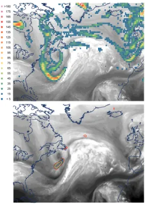
(Fig.1b), the BL tracer valid 2 days prior to the observation ranges from 50% to 65%. It mainly implies the origin of WCB1 in the planetary boundary layer. The positions of particles of WCB1 2 days prior to the observation are plotted on a composite im-age of water vapor radiance from GEOS-East and METEOSAT, and with the ECMWF geopotential field at 1000 hPa (Fig. 2a). At that time, particles of WCB1 are located 10

in the warm sector of a maritime cyclone. Later on, as the surface cyclone intensifies and moves northeastward, particles of WCB1 enter in the warm conveyor belt of that cyclone and ascend in the free troposphere.

The residence time of particles of WCB1 in the free troposphere is about two days. It includes the transport by the WCB and by the upper-tropospheric ridge ahead of 15

the surface cyclone. Ascending trajectories of the WCB1 particles interleave over the subsiding trajectories of the FOLD1 particles over Frankfurt.

The BL tracer associated with WCB2 is shown 5.75 days prior to the observation (Fig. 1b). It ranges from 50% to 55%, mainly implying a planetary boundary layer origin. Positions of WCB2 particles at that time are presented on the composite picture 20

made with satellite radiances and the 1000-hPa geopotential field (Fig.2b). The group of particles of WCB2 that is located south of Newfoundland is embedded in the WCB of a surface cyclone growing along the East Coast of USA. Its residence time in the free troposphere, after extraction from the marine boundary layer and up to the time of observation in Frankfurt, is about 5 days. East of Newfoundland, backward trajectories 25

show a second group of particles associated with WCB2. This group has not been embedded in a WCB during its life cycle and participates in the mixing of WCB2.

(11)

ACPD

7, 1119–1142, 2007

J. Brioude

Title Page

Tables Figures

◭ ◮

Back Close

Full Screen / Esc

EGU

prior to the observation time are shown on Fig. 1. The investigation of a possible stratospheric-origin of FOLD2 continues in the section below in which a clustering method is used to better characterize the life cycle of some of the FOLD2 particles.

3.2 Capture of stratospheric-origin signatures

At a time of 6.75 days prior to the MOZAIC observations, the retroplume initialized with 5

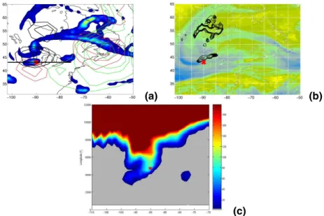
particles in the FOLD2 layer (colored contours on Fig.3a) shows a large geographical dispersion from 50◦W to 100◦W. This retroplume is composed of three main groups of particles. The first group lies between 0.5 and 5 km altitude and stretches along the eastern coast of north America (centre at about 60◦W–50◦N, see red and green contours). The second group lies between 3 and 10 km altitude west and south-west 10

of the Great Lakes (red and black contours). The third group lies between 5 and 10 km altitude west of Hudson Bay (black contours). The 5-km stratospheric-ozone tracer, based on the Flexpart run in the forward mode and used to prescribe the ozone mixing ratio of advected particles of stratospheric-origin, is shown on Fig.3a (see the colored field). It shows the structure of a wave in the mid-troposphere.

15

According to the method to prescribe an ozone mixing ratio to stratospheric-origin particles, it can be seen on Fig.3b that none of the particles of the first group of the FOLD2 retroplume is associated with a possible stratospheric-origin. However, the second and third groups of the FOLD2 retroplume have got a stratospheric-origin. Par-ticles of stratospheric-origin associated with the second group of the FOLD2 retroplume 20

lie at the eastern tip of a dry band in the water vapour image (Fig.3b) They belong to the upper-level dynamical precursor that triggers the development of the surface low involved in the formation of the WCB2 layer (see Fig.2b). One of the ten clusters of the FOLD2 retroplume which is valid at the same date has an altitude of 4.7 km, a PV of 1.4 pvu, a relative humidiy of 25% and a mass fraction of 3%. The characteristics of 25

(12)

ACPD

7, 1119–1142, 2007

J. Brioude

Title Page

Tables Figures

◭ ◮

Back Close

Full Screen / Esc

EGU

frame of the stratospheric-ozone tracer, the stratospheric ozone vertical cross section on Fig. 3c confirms that this cluster lies in an ozone structure (with an ozone mixing ratio of about 90 ppbv) that illustrates the presence of an upper level trough.

The third group of the FOLD2 retroplume, which has been shown to be of stratospheric-origin, lies in a large tropopause disturbance as indicated by the dry ar-5

eas on the water vapor satellite image (Fig.3b). In the course of the development of the surface low associated with the FOLD2 and WCB2 features, particles of the third group of the FOLD2 retroplume will finally catch up and merge with particles of the second group. The stratospheric intrusion process is shown at a later time period, i.e. 5.75 days (Fig.2b) and 4.75 days (Fig.4) prior to the MOZAIC observations. The stratospheric 10

ozone tracer (Fig.4a) fills up the two dry airstreams associated with the development of the surface low. The RDF-ozone field shows that only the northern dry airstream is associated with the development of FOLD2. Note that because of the descent of the stratospheric intrusion, both the stratospheric ozone tracer and the RDF-ozone fields were shown at 4 km altitude. To complete the documentation of the life cycle of FOLD2, 15

the RDF-ozone relative to FOLD2 is shown on Fig.2b at the time of extraction of the WCB2 particles out of the marine boundary layer into the free troposphere, i.e. 5.75 days prior to the observations. Again, the position of the RDF-ozone feature in the dry air stream of the surface low is an evidence of stratospheric-origin of FOLD2.

3.3 Reconstruction of the ozone profile 20

In this section, we use the FLEXPART RDF-ozone simulation to reconstruct the ozone profile over Frankfurt, and to assess the residence time of the tropopause fold FOLD2 in the troposphere. The reconstruction of the RDF-ozone values along the MOZAIC profile is based on the initialisation of the stratospheric ozone tracer above 7 km al-titude to only take into account stratospheric features in the UTLS domain. Figure5 25

(13)

ACPD

7, 1119–1142, 2007

J. Brioude

Title Page

Tables Figures

◭ ◮

Back Close

Full Screen / Esc

EGU

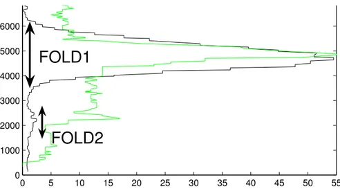
RDF-ozone peak of 55 ppbv, which confirms its stratospheric origin. On the lower part of the profile, though the RDF-ozone is weak, a maximum of 3 ppbv coincides with the FOLD2 layer. It constitutes a signature of the stratospheric-origin of FOLD2. The RDF-ozone peak is smaller and broader than the RDF-ozone peak from measurements. The use of analyzed fields can result in an overestimation of mixing between air masses (Stohl 5

et al., 2004). The parametrization of turbulence into the model can also contribute to spread the peak. Such a stratospheric signature in the RDF-ozone simulation lasts during the period from 6.5 to 7.5 days prior to the measurements. An assessment of the residence time of tropopause fold FOLD2 into the tropopshere is therefore about 6.5 days. Finally, the RDF-ozone technique has allowed us to attribute a stratospheric-10

origin to FOLD2, and to assess a residence time in the troposphere of about 6.5 days. This residence time is also characteristics of the period of time for a complete mixing of the stratospheric-origin layer into the troposphere because FOLD2 can be considered as a very weak ozone anomaly (₊8 ppbv compared to the tropospheric background on the vertical profile) that will likely disappear by venting and turbulence effects at the top 15

of the boundary layer.

4 Conclusions

A lagrangian analysis has been made with the FLEXPART Lagrangian particle disper-sion model to characterize the tropospheric layering revealed by a vertical profile of ozone, carbone monoxide and relative humidity observed over Frankfurt (Germany) 20

by one of the commercial airliner participating to the MOZAIC programme. It demon-strates the interleaving along the vertical profile of 4 coherent airstreams, two warm conveyor belts and two tropopause folds, that are characteristic of the dynamics of mid-latitude extratropical lows. Layers associated with the two warm conveyor belts are centred at 3 km and 7 km altitude. They are relatively thick (2 to 3 km in altitude) 25

(14)

ACPD

7, 1119–1142, 2007

J. Brioude

Title Page

Tables Figures

◭ ◮

Back Close

Full Screen / Esc

EGU

They are representative of particles being extracted from the maritime boundary layer into the free troposphere by warm conveyor belts ahead of surface cold fronts over the Atlantic. According to Flexpart simulations, their residence time into the troposphere range from 2 to 5.75 days. The first tropopause fold is observed at 4.7 km altitude. It is about 1 km deep and has retained strong stratospheric-origin signatures, i.e. 95 ppbv 5

for ozone, 70 ppbv for carbon monoxide and 10% for relative humidity. The residence time of the fold into the troposphere is about 2 days at the time of the observation. The second tropopause fold is a few hundred metres deep and is observed at 2.2 km altitude just above the planetary boundary layer. Stratospheric-origin signatures are very weak and mainly consist in the anti-correlation of relative anomalies of ozone and 10

carbone monoxide volume mixing ratios (₊8 ppbv and –5 ppbv, respectively) compared to the tropospheric background. According to the Flexpart simulations, its residence time into the free troposphere is about 6.5 days as the folding process occured over northeastern America. This period of time is also representative of the time scale for a complete mixing of the tropopause fold into the troposphere.

15

The interests for such a case study are to illustrate in a Lagrangian context the diverse origin of laminae. The free troposphere of this case study is characterized by four interleaved layers which were processed by coherent airstreams coming from frontal systems. This case study exemplifies the diverse origin that may be ascribed to the ubiquitous tropospheric laminae identified by Newell et al. (1999).

20

A Reverse Domain Filling technique, combining a simulation of stratospheric ozone in a forward mode and back trajectories, has been proposed to prescribe ozone mixing ratio to stratospheric-origin particles.

Our method has been successfully used to demonstrate the stratospheric-origin of the two tropopause folds and to lengthen the period of time on which to assess the res-25

(15)

ACPD

7, 1119–1142, 2007

J. Brioude

Title Page

Tables Figures

◭ ◮

Back Close

Full Screen / Esc

EGU

systematic application on the MOZAIC data base which contains more than 28 000 ver-tical profiles from 1994 to 2006, as tentatively begun by Zbinden et al. (2006). It would allow a climatological characterization of the layering structure of the troposphere and improvments in the assessment of the contribution of the stratospheric flux on the tro-pospheric ozone budget

5

Acknowledgements. Satellite data were provided by the SATMOS service (http://www.

satmos-meteo.fr/) and by O. Cooper (NOAA, Boulder). The authors acknowledge the Euro-pean Communities and EADS-Airbus for their strong support to the MOZAIC programme, and the particpating airlines (Lufthansa, Austrian, Air France) for the transport and the maintennace of the equipment free of charge since 1994.

10

References

Appenzeller, C., Holton, J. R., and Rosenlof, K. H.: Seasonal variation of mass transport across the tropopause, J. Geophys. Res., 101(D10), 15 071–15 078, 1996.

Beuermann, J., Konopka P., Brunner D., Bujok O., Gunther O., McKenna D.S., Lelieveld J., Muller R., and Schiller C.: Highresolution measurements and simulation of stratospheric and

15

tropospheric intrusions in the vicinity of the polar jet stream, Geophys. Res. Lett., 29(12), 1577, doi:10.29/2001GL014162, 2002.

Bithell, M., Gray, L .J., and Cox, B. D.: A three-dimensional view of the evolution of midlatitude stratospheric intrusions, J. Atmos. Sci., 56, 673–687, 1999.

Bithell, M., Vaughan, G., and Gray, L. J.: Persistence of stratospheric ozone layers in the

20

troposphere, Atmos. Environ., 34(16), 2563–2570, 2000.

Brioude J., Cammas, J.-P., and Cooper O. R.: Stratosphere-troposphere exchange in a sum-mertime extratropical low: analysis, Atmos. Chem. Phys., 6, 2337–2353, 2006,

http://www.atmos-chem-phys.net/6/2337/2006/.

Colette, A. and Ancellet, G.: Impact of vertical transport processes on the tropospheric ozone

25

layering above Europe. Part II: Climatological analysis of the past 30 years, Atmos. Env., 39, 5423–5435, 2005.

(16)

ACPD

7, 1119–1142, 2007

J. Brioude

Title Page

Tables Figures

◭ ◮

Back Close

Full Screen / Esc

EGU

distributions over three North American sites, J. Geophys. Res., 103(D17), 22 001–22 013, 1998.

Cooper, O. R., Moody, J. L., Parrish, D. D., Trainer, M., Ryerson, T. B., Holloway, J. S., Hubler, G., Fehsenfeld, F. C., Oltmans, S. J., and Evans, M. J.: Trace gas signatures of the airstreams within North Atlantic cyclones: Cases Studies from the North Atlantic Regional Experiment

5

(NARE’97) aircraft intensive, J. Geophys. Res., 106(D6), 5437–5456, 2001.

Cooper, O. R., Moody, J. L., Parrish, D. D., Trainer, M., Ryerson, T. B., Holloway, J. S., Hubler, G., Fehsenfeld, F. C., and Evans, M. J.: Trace gas composition of midlatitude cyclones over the western North Atlantic Ocean: A conceptual model, J. Geophys. Res., 107(D7), 4056, doi:10.1029/2001JD000901, 2002a.

10

Cooper, O. R., Moody, J. L., Parrish, D. D., Trainer, M., Holloway, J. S., Hubler, G., Fehsenfeld, F. C., and Stohl, A.: Trace gas composition of mid-latitude cyclones over the western North Atlantic Ocean: A seasonal comparison of ozone and CO, J. Geophys. Res., 107(D7), 4057, doi:10.1029/2001JD000902, 2002b.

Cooper, O. R., Forster, C., Parrish, D., Dunlea, E., Hubler, G., Fehsenfeld, F., Holloway, J.,

Olt-15

mans, S., Johnson, B., Wimmers, A., and Horowitz, L.: On the life-cycle of a stratospheric in-trusion and its dispersion into polluted warm conveyor belts, J. Geophys. Res., 109, D23S09, doi:10.1029/2003JD004006, 2004.

Cooper, O. R., Stohl, A., Hubler, G., Hsie, E. Y., Parrish, D. D., Tuck, A. F., Kiladis, G. N., Oltmans, S. J., Johnson, B. J., Shapiro, M., Moody, J. L., and Lefohn, A. S.: Direct transport

20

of midlatitude stratospheric ozone into the lower troposphere and marine boundary layer of the tropical Pacific Ocean, J. Geophys. Res., 110, D23310, doi:10.1029/2005JD005783, 2005.

Curtius, J., Sierau, B., Arnold, F., de Reus, M., Str ¨om, J., A. Scheeren, H., and Lelieveld, J.: Measurement of aerosol sulfuric acid 2. Pronounced layering in the free troposphere

dur-25

ing the second Aerosol Characterization Experiment (ACE 2), J. Geophys. Res., 106(D23), 31 975–31 990, doi:10.1029/2001JD000605, 2001.

Danielsen, E. F.: Stratospheric-tropospheric exchange based upon radioactivity, ozone and potential vorticity, J. Atmos. Sci., 25, 502–518, 1968.

Eckhardt, S., Stohl, A., Wernli, H., James, P., Forster, C., and Spichtinger N.: A 15-Year

clima-30

tology of Warm Conveyor Belts, J. Climate, 17, 218–237, 2004.

(17)

ACPD

7, 1119–1142, 2007

J. Brioude

Title Page

Tables Figures

◭ ◮

Back Close

Full Screen / Esc

EGU

Esler, J. G., Tan, D. G. H., Haynes, P. H., Evans, M. J., Law, K. S., Plantevin, P. H., and Pyle, J. A.: Stratosphere-troposphere exchange: Chemical sensitivity to mixing, J. Geophys. Res., 106(D5), 4717–4731, doi:10.1029/2000JD900405, 2001.

Esler, J. G., Haynes, P. H., Law, K. S., Barjat, H., Dewey, K., Kent, J., Schmitgen, S., and Brough, N.: Transport and mixing between airmasses in cold frontal regions

dur-5

ing Dynamics and Chemistry of Front Zones (DCFZ), J. Geophys. Res., 108(D4), 4142, doi:10.1029/2001JD001494, 2003.

Forster, C. and Wirth, V.: Radiative decay of idealized stratospheric filaments in the tropo-sphere, J. Geophys. Res., 105, 10 169–10 184, 2000.

Gray L. J., Bithell, M., and Cox, B. D.: The role of specific humidity fields in the diagnosis of

10

stratosphere troposphere exchange, Geophys. Res. Lett., 21, 2103–2106, 1994.

Hegglin, M. I., Brunner, D., Wernli, H., Schwierz, C., Martius, O., Hoor, P., Fischer, H., Par-chatka, U., Spelten, N., Schiller, C., Krebsbach M., Weers, U., Staehelin, J., and Peter, Th.: Tracing troposphere-to-Stratosphere transport above a mid-latitude deep convective system, Atmos. Chem. Phys., 4, 741–756, 2004,

15

Legras B., Joseph B., and Lefevre F.: Vertical diffusivity in the lower stratosphere from

La-grangian back-trajectory reconstructions of ozone profiles, J. Geophys. Res., 108(D18), 4562, doi:10.1029/2002JD003045, 2003.

Mahfouf J.-F. and Rabier, F.: The ECMWF operational implementation of four dimensional

vari-20

ational assimilation. Part II: Experimental results with improved physics, Quart. J. Roy. Me-teorol. Soc., 126, 1171–1190, 2000.

Marenco, A., Thouret, V., Nedelec, P., Smit, H., Helten, M., Kley, D., Karcher, F., Simon, P., Law, K., Pyle, J., Poschmann, G., Von Wrede, R., Hume, C., and Cook, T.: Measurement of ozone and water vapor by Airbus in-service aircraft: The MOZAIC airborne program, An overview,

25

J. Geophys. Res., 103, 25 631–25 642, 1998.

Methven, J., Arnold, S. R., O Connor, F. M., Barjat, H., Dewey, K., Kent, J., and Brough, N.: Estimating photochemically produced ozone throughout a domain using flight data and a Lagrangian model, J. Geophys. Res., 108(D9), 4271, doi:10.1029/2002JD002955, 2003. Nedelec, P. , Cammas, J. -P., Thouret, V., Athier, G., Cousin, J. -M., Legrand, C., Abonnel,

30

(18)

ACPD

7, 1119–1142, 2007

J. Brioude

Title Page

Tables Figures

◭ ◮

Back Close

Full Screen / Esc

EGU

Newell, R. E., Thouret, V., Cho, J. Y. N., Stoller, P., Marenco, A., and Smit, H. G.: Ubiquity of quasi-horizontal layers in the troposphere, NATURE, 398, 316–319 doi:10.1038/18,642, 1999.

Rabier, F., Jarvinen, H., Klinker, E., Mahfouf, J.-F., and Simmons, A.: The ECMWF operational

5

implementation of fourdimensional variational assimilation. Part I: Experimental results with simplified physics, Quart. J. Roy. Meteorol. Soc., 126, 1143–1170, 2000.

Shapiro, M. A.: Further evidence of the mesoscale and turbulent structure of upper level jet stream-frontal zone systems/ Mon. Wea. Rev., 106, 1100–1111, 1978.

Shapiro, M. A.: Turbulent mixing within tropopause folds as a mechanism for the exchange of

10

chemical constituents between the stratosphere and troposphere, J. Atmos. Sci., 37, 994– 1004, 1980.

Stohl, A. and Thomson, D. J.: A density correction for Lagrangian particle dispersion models, Boundary Layer Meteorol., 90, 155–167, 1999.

Stohl, A. and Trickl, T.: A textbook example of long-range transport: Simultaneous observations

15

of ozone maxima of stratospheric and North American origin in the free troposphere over Europe, J. Geophys. Res., 104(30), 445–462, 1999.

Stohl, A., Spichtinger-Rakowsky, N., Bonasoni, P., Feldmann, H., Memmesheimer, M., Scheel, H. E., Trickl, T., Hbener, Hubener, S., Ringer, W., and Mandl, M.: The influence of strato-spheric intrusions on alpine ozone concentrations, Atmos. Environ., 34, 1323–1354, 2000.

20

Stohl, A.: A one year Lagrangian climatology of airstreams in the Northern Hemisphere tropo-sphere and lowermost stratotropo-sphere, J. Geophys. Res., 106, 7263–7279, 2001.

Stohl, A., Eckhardt, S., Forster, C., James, P., Spichtinger, N., and P.,: A replacement for simple back trajectory calculations in the interpretation of atmospheric trace substance measure-ments, Atmos. Environ. 36, 4635–4648, 2002.

25

Stohl, A., Bonasoni, P., Cristofanelli, P., Collins, W., et al.: Stratosphere-Troposphere exchange: A review, and what we have learned from STACCATO, J. Geophys. Res., 108(D12), 8516, doi:10.1029/2002JD002490, 2003.

Stohl, A., Cooper, O. R., and James, P.: A cautionary note on the use of meteorological analysis fields for quantifying atmospheric mixing, J. Atmos. Sci., 61(12), 1446–1453, 2004.

30

Stohl, A., Forster, C., Frank, A., Seibert, P., and Wotawa, G.: Technical Note : The Lagrangian particle dispersion model FLEXPART version 6.2, Atmos. Chem. Phys., 5, 2461–2474, 2005,

(19)

ACPD

7, 1119–1142, 2007

J. Brioude

Title Page

Tables Figures

◭ ◮

Back Close

Full Screen / Esc

EGU

Thouret, V., Marenco, A., Nedelec, P., and Grouhel, C.: Ozone climatologies at 9–12 km altitude as seen by the MOZAIC airborne program between September 1994 and August 1996, J. Geophys. Res., 103, 25 653–25 679, 1998.

Thouret, V., Cho, J. Y. N., Newell, R. E., Marenco, A., and Smit, H. G. J.: General characteristics of tropospheric trace constituent layers observed in the MOZAIC program, J. Geophys. Res.,

5

105(D13), 17 379–17 392, 2000.

Vaughan G., Price, J. D., and Howells, A.: Transport into the troposphere in a tropopause fold, Q. J. R. Meteorol. Soc., 120, 1085–1103, 1994.

Volz-Thomas, A., Berg, M., Heil, T., Houben, N., Lerner, A., Petrick, W., Raak, D., and Patz, H.-W.: Measurements of total odd nitrogen (NOy) aboard MOZAIC in-service aircraft:

instru-10

ment design, operation and performance, Atmos. Chem. Phys., 5, 583–595, 2005,

Wernli, H. and Davies, H. C.: A Lagrangian-based analysis of extratropical cyclones. I: The method and some applications, Q. J. Roy. Meteorol. Soc., 123, 467–489, 1997.

Wernli, H. and Bourqui, M.: A one-year Lagrangian climatology of (deep) cross-tropopause

15

exchange on the extratropical northern hemisphere, J. Geophys. Res., 107, 4021, doi:10.1029/2001JD000812, 2002.

Zbinden, R. M., Cammas, J.-P., Thouret, V., Nedelec, P., Karcher, F., and Simon, P.: Mid-latitude tropospheric ozone columns from the MOZAIC program: climatology and interannual variability, Atmos. Chem. Phys., 6, 1053–1073, 2006,

20

(20)

ACPD

7, 1119–1142, 2007

J. Brioude

Title Page

Tables Figures

◭ ◮

Back Close

Full Screen / Esc

EGU

0 20 40 60 80 100

0 1000 2000 3000 4000 5000 6000 7000 8000 9000 10000

O

3(ppbv), RH(%)

0 50 CO(ppbv)100 150

WCB1

FOLD1

WCB2

FOLD2

(a) 0 20 40 60 80 100

0 1000 2000 3000 4000 5000 6000 7000 8000 9000 10000

ST(%), BL(%) WCB2

WCB1

FOLD1

(b)

Fig. 1. (a)MOZAIC vertical profile over Frankfurt on 10 February 2002, 12:00 UTC for ozone

(ppbv, black line), CO (ppbv, red line) and relative humidity (%, green line) versus barometric

altitude (m). (b)Fractions of boundary layer (BL) tracer (%, star) and stratospheric (ST) tracer

(21)

ACPD

7, 1119–1142, 2007

J. Brioude

Title Page

Tables Figures

◭ ◮

Back Close

Full Screen / Esc

EGU

Fig. 2. Composite pictures of water vapour channel radiances (converted in temperatures, K)

for GOES-EAST and METEOSAT satellites, and 1000-hPa geopotential fields from ECMWF analyses valid on

(a)8 February, 12:00 UTC (2 days prior to the observation time) and

(b)4 February, 18:00 UTC (5.75 days prior to the time of observation).

(22)

ACPD

7, 1119–1142, 2007

J. Brioude

Title Page

Tables Figures

◭ ◮

Back Close

Full Screen / Esc

EGU

(a) (b)

(c)

Fig. 3. Stratospheric-origin indicators relative to the formation of the FOLD2 layer observed in

Frankfurt (Fig.1). All fields are valid on 3 February, 18:00 UTC (6.75 days prior to the time of

observation).

(a)Stratospheric ozone tracer (coloured field, ppbv, colobar in c) at 5 km altitude as derived

from the Flexpart simulation in the forward mode. Contours represent the percentages (0.05%, 0.1%, 0.25%, 0.5%, and 1.5%) of air particles associated with the retro-plume of the FOLD2 layer. Green, red and black contours are for particles with end-of-trajectory altitudes in the layers 0.5–3 km, 3–5 km, and 5–10 km, respectively. The red cross indicates the position of the cluster of particles described in the text.

(b)Radiances in the water vapor channel of GOES-EAST (colored field, K). Black contours

represent the contribution of the stratospheric ozone tracer (0.01, 0.015, 0.02, 0.025, and 0.03 ppbv contours) prescribed to the RDF-ozone of layer FOLD2.

(23)

ACPD

7, 1119–1142, 2007

J. Brioude

Title Page

Tables Figures

◭ ◮

Back Close

Full Screen / Esc

EGU

(a)

(b)

< 5 1 5 2 5 3 5 4 5 5 5 6 5 7 5 8 5 9 5 1 0 5 1 1 5 1 3 5 1 5 5 1 7 5

1 2 5 1 4 5 1 6 5 > 1 8 0

Fig. 4. GOES-EAST and METEOSAT satellites radiance temperature (K) in the water vapour

channel on 5 February, 18:00 UTC (4.75 days prior to the time of observation).

(a) Stratospheric-ozone tracer field (ppbv, colored square) at 4 km altitude derived from the

forward mode of the Flexpart simulation.

(b)Contours represent the contribution of the stratospheric ozone tracer (0.01, 0.015, 0.02,

(24)

ACPD

7, 1119–1142, 2007

J. Brioude

Title Page

Tables Figures

◭ ◮

Back Close

Full Screen / Esc

EGU

0 5 10 15 20 25 30 35 40 45 50 55

0 1000 2000 3000 4000 5000 6000 7000

FOLD1

FOLD2

Fig. 5. MOZAIC vertical profile for ozone as observed in Frankfurt on 10 February, 12:00 UTC