ISSN-1139-3394
DOI:10.3369/tethys.2006.3.04
Numerical Modelling of Troposferic Ozone in Catalunya
S.Ortega1, M.R. Soler1, J. Beneito1, and D. Pino2,3
1Department of Astronomy and Meteorology, University of Barcelona, Avd. Diagonal 647, 08028 Barcelona 2Institute for Space Studies of Catalonia, Edifici Nexus 2, Gran Capit`a 2-4, 08034 Barcelona
3Applied Physics Departament, Technical University of Catalonia, Avd. Del Canal Ol´ımpic s/n, 08860 Castelldefels,
Barcelona
Received: 22-V-2006 – Accepted: 23-XI-2006 –Original version
Correspondence to:rosa@am.ub.es
Abstract
The aim of this paper is to evaluate the ability of two different modelling systems to simulate high values of ozone concentration in typical summer episodes which take place in Catalonia, located in the north-east part of Spain. The first model, or forecasting system, is a box model made up of three modules. The first module is a mesoscale model (MASS), which provides the initial condition for the second module, a non-local boundary layer model based on the transilient turbulence scheme. The third module is a photochemical box model (OZIPR), which is applied in Eulerian and Lagrangian modes receiving suitable information from the two previous modules. The model forecast is applied to different areas of Catalonia and evaluated during the springs and summers of 2003 and 2004 against ground base stations. The second model is MM5/UAM-V, a grid model designed to predict the hourly three-dimensional ozone concentration fields. The model is applied during an ozone episode occurred between 21 and 23 June 2001 at only one area, which is characterized by complex topography and a peculiar meteorological condition favouring high ozone concentration values. Evaluation results and model comparison for this specific episode show a good performance of the two modelling systems.
1 Introduction
Ozone has recently become a problem pollutant in both industrial and rural areas of southern Europe (Silibello et al., 1998; Grossi et al., 2000) during spring and summer. It is associated with increasing emissions of nitrogen oxides and organic compounds, which, activated by solar radiation, pro-duce ozone in the planetary boundary layer. Evidence of it is provided by the elevated ozone concentrations measured in the last few decades in urban and industrial areas and es-pecially in many downwind rural areas, where local ozone precursors are lacking.
For several reasons, tropospheric ozone is considered to be one of the worst pollutants in the lower troposphere. A higher concentration of tropospheric ozone can contribute to a potentially important climate forcing, which needs to be properly assessed (Chalita et al., 1996). It is toxic to plants so it reduces crop yields (Guderian et al., 1985; Hewit et al., 1990). To humans it acts as a respiratory irritant that reduces lung function (Lippmann, 1991). It also damages both natu-ral and artificial materials such as stone, brickwork and
rub-ber. Controlling and forecasting ozone concentrations can therefore benefit humans, vegetation and the economy. This control is also needed for assessing the scale of ozone im-pacts and for developing control strategies through appropri-ate measurements and modelling.
In the last three decades, significant progress has been made in air-quality modelling systems. The simple Eulerian box models have evolved into complex variable-grid models. The early box models were a first approach to incorporating the complex chemistry that links primary and secondary pol-lutants and to including some meteorological variables, but they were an oversimplification of the processes and mecha-nisms that act in the troposphere. The Lagrangian box mod-els were improvements of the Eulerian box modmod-els because the column of air (the box) moved along the trajectory of certain initial pollutant concentrations. In fact, they were an expansion of the simple box model to a series of adjacent, interconnected boxes.
kind of model takes into account interactions between the different cells and involves many physical and chemical pro-cesses but requires a complete description of the zone in which they are applied. This is usually more extensive than in box models, which makes it more difficult to obtain suc-cessful results.
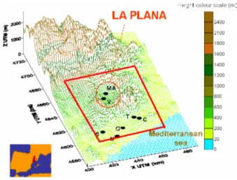
Today many photochemical models are applied in dif-ferent parts of the world. Sufficient good results have been obtained in the modelling of tropospheric ozone. However, few models have been used in Catalonia (NE Spain), which has important industrial areas on the coast around Barcelona and Tarragona. These areas act as an important anthro-pogenic source of ozone and precursors, which increases the air pollution, especially of ozone, in neighbouring areas. One of the most problematic is called La Plana. This is a topo-graphically complex area northeast of Barcelona (see section 2 for a detailed description). One of the causes of this in-creased air pollution, apart from its own production, is pollu-tant advection from the area of Barcelona to La Plana via sea breeze, which penetrates further inland to reach the whole area. La Plana also frequently presents stagnating meteo-rological conditions that, coupled with high solar radiation, lead to maximum ozone levels that exceed the threshold pre-scribed. This is why in this study we apply two different models to this area to forecast ozone concentration and to compare model performances.
The first modelling system is a photochemical box model (OZIPR), which has been applied in an Eulerian and Lagrangian modes. Beside, this modelling system is inte-grated by a meteorological module composed by a mesoscale model (MASS) which provides the trajectory followed by the box model when it is applied in a Lagrangian mode and the initial condition to a non local boundary layer model based on the transilient turbulence scheme model.
The second modelling system is made up of a three-dimensional grid-based photochemical model (UAM-V) ap-plied in a non-nested mode and a mesoscale model (MM5) that provides the meteorological conditions for the photo-chemical model. This system was applied in a small domain covering part of the industrial zone near Barcelona and the whole of La Plana, where high ozone levels are frequently observed.
The importance of emissions in photochemical models is well known. For this reason an emission model covering the whole area in which the models were applied was inte-grated in order to supply the corresponding emissions from surface and elevated sources.
Section 3 presents a detailed description of both mod-elling systems. Section 4 describes the emission model. Sec-tion 5 presents model applicaSec-tion results, which are discussed and validated while section 6 compares the models. Finally, section 7 provides some concluding remarks.
Figure 1. Topographic map of Catalonia, contour intervals are labelled every 200m. Ozone concentration has been forecasted in the areas delimited by a rectangle.
2 The experiment
2.1 The studied areas
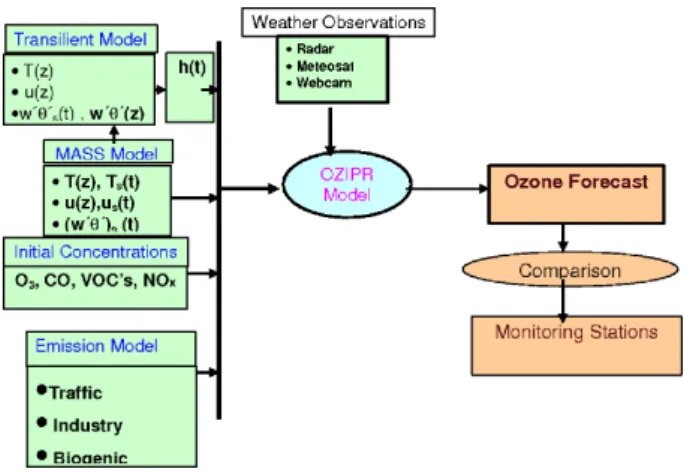
Figure 2.Diagram of the box modelling components.
Empord`a Plain where there is an important motorway, AP-7, which during summer holidays could generate high values of ozone concentration.
2.2 Meteorological and air pollution data
In this study we used data from several meteorologi-cal and air quality ground stations belonging to a network of surface stations. Every 30 minutes they provide data about solar radiation, temperature, wind speed and direction, rel-ative humidity, and CO, NO, NO2 and O3 concentrations.
To validate the box model a representative monitoring sta-tion located in Alcover (area 1), Vilanova i la Geltr´u (area 2), Vic and Pardines (areas 3 and 4) and Agullana (area 5) have been selected. To validate the Eulerian model we used data from Sabadell (S), Granollers (G), St Celoni (C), Sta. Maria de Palautordera (T), Vic (V), Manlleu (MA) and Mollet (M), which are located inside and outside the La Plana region (see Figure 4).
3 Modelling systems
3.1 Box model
The box modelling system is made up of three fun-damental modules containing two meteorological models, a column or a box photochemical model and an emission model, respectively -a schematic diagram is presented in Figure 2. In this section we will briefly describe the first two modules and in section 4 we will describe the emission model, which is shared by the two modelling systems.
The meteorological module comprises two models. The first one was an upgrade of the Mesoscale Atmospheric Simulation System, hereafter referred to as MASS (Kaplan et al., 1982; Zack and Kaplan, 1987), which is the opera-tional model of the Catalan Weather Service. The second one was a 1-D atmospheric boundary layer (ABL) model based on transilient turbulence scheme (Stull, 1984a,b).
MASS is a 3-dimensional hydrostatic primitive mesoscale model executed with two domains one way nested, which are defined using resolutions of 30 and 8 km. The dimensions of each domain are 55 x 55 grid points for the outer domain and 103 x 103 grid points for the inner domain. The biggest domain is centred at (40.0◦ N, 10.0◦ E) and the smallest domain is centred at (41.0◦ N, 3.0◦ W), covering an area from 37.5◦ N to 44.5◦ N. The initial and boundary conditions are updated every six hours with information from the AVN model with a 0.55◦x 0.55◦ resolution. For both domains, we used a topography and land-use date base with 10 min resolution. High vertical resolution is prescribed in the ABL with 21 levels, with higher resolution on the lower levels. More information about model physics and numerics are described in Codina et al. (1997).
The 1-D atmospheric boundary layer model is based on the non-local transilient turbulence closure (Stull, 1984a,b), which was first developed by R. B. Stull as an alternative to local closure schemes such as K-theory and higher-order closure. In this approach, we used the matrix of mixing (transilient) coefficients developed by Stull and Driedonks (1987) and calculated from a simplified form of turbulence kinetic energy. In the model, each time step is split into two parts. In the first one, external forcing (e.g. the dynamics, thermo-dynamics, boundary conditions) destabilize the flow, and in the second one the transilient turbulence scheme reacts to instabilities via mixing. In this way mean wind, potential temperature and specific humidity are destabilized by momentum and sensible and latent heat fluxes from the ground. Surface momentum fluxes are calculated using the drag coefficient method, while sensitive and latent heat fluxes are calculated using the (Blackadar, 1976, 1979) surface model. In addition, turbulence profiles of kinematic turbulent fluxes are calculated using the transilient turbulent closure scheme. With this information we were able to calculate the height of the boundary layer, defined as the height of most negative heat flux or as the average base of the overlying stable layer. The height of the boundary layer is the height of the photochemical box model. It is therefore very important to correctly estimate it in order to determine the ozone concentration (Berman et al., 1997).
The photochemical model used in this study was the OZIPR model (Ozone Isopleth Plotting Programme, Research), (Gery and Crouse, 1990). This is a column or a box model developed by the EPA (Environmental Protection Agency). It is a single day forecast model designed to focus on the atmospheric chemistry that leads to ozone formation. The chemical mechanism we used in this paper was the carbon bond approach (Gery et al., 1989; Stockwell et al., 1990). Dry deposition at the surface is included in the model in a simple way. For each species, values are fixed for two types of surface urban and rural.
are included during the day. The model is run in Eulerian and Lagrangian modes. In the first mode, the air mass, which is taken as 20 x 20 km2over a region, is treated as a box in which pollutants are emitted. Transport into and out of the box by meteorological processes and dilution is taken into account. However, in this Eulerian mode, mesoscale effects such as sea breeze are not considered. To take this into account, therefore, the box model must be applied in the Lagrangian mode following the trajectory, which is calculated using a back trajectory model (Alarc´on et al., 1995; Alarc´on and Alonso, 2001). For more accurate information to obtain trajectories than those provided by MASS model (horizontal resolution 8 km), the MM5 model with a 1 km resolution is run. In the Lagrangian mode this idealized column moves with the wind (along the air mass trajectory), but cannot expand horizontally. Emissions are included as the air column passes over different emission sources, since the hourly emissions into the air mass were taken from the 3 x 3 km2grid-based emission list. With the Lagrangian simulation the incoming ozone to the idealized columns is taken into account as an ozone advection. In both simulations air from above the column is mixed in as the inversion rises during the day and dilution occurs during the simulation, in which chemical reactions are converting the VOC and NOx to O3and other secondary pollutants.
As well as initial concentrations and hourly emissions, other inputs in the OZIPR model are temperature, relative humidity and mixing height, which is the height of the column model. The hourly evolution of the mixing height is one of the critical parameters of the calculations needed for the OZIPR model, as the rate of dilution of atmospheric pollutants is controlled by the diurnal change in mixing height.
3.2 Grid model
The other modelling system used is the MM5 meteo-rological model coupled with the photochemical model Ur-ban Airshed Model (UAM-V), version 1.30 (fast chemistry solver), which has been widely used for regulatory purposes (Biswas et al., 2001).
UAM-V uses meteorological data provided by the Penn State University/National Center of Atmospheric Research mesoscale Model (MM5), version 3.4 (Grell et al., 1994). Four domains two ways nested are defined using the follow-ing resolution: 27, 9, 3 and 1 km. To simulate the sea breeze, the dimensions of each domain are 31 x 31 grid points for the two outer domains, and 37 x 43 and 37 x 61 grid points for the two inner domains, respectively. The biggest domain is centred at (41.70◦N, 2.27◦E) and the smallest domain cov-ers an area from 41.6◦ N to 42.1◦ N (figure 3). The initial and boundary conditions are updated every six hours with information from the European Centre for Medium Range Weather Forecast (ECMWF) model with a 0.5◦x 0.5◦ reso-lution. For the two inner domains, we used a topography and
Figure 3. The 4 domains of the MM5 simulation. The inner do-main is the same used by UAMV.
land-use date base with 30” resolution. For the two outer do-mains the horizontal resolution was 5’. High vertical resolu-tion is prescribed in the atmospheric boundary layer with 14 levels. More details about the performance of the MM5 can be found in Soler et al. (2003). The meteorological outputs of the smallest domain are made compatible with the UAM-V grid configuration by performing interpolations along the horizontal and vertical levels.
The UAM-V modelling system employs an updated ver-sion of the original Carbon Bond IV chemical kinetics anism (Gery et al., 1989), which contains the CB-TOX mech-anism (Ligocki and Whitten, 1992; Ligocki et al., 1992). In addition to the isoprene update, this includes an expanded chemical treatment for aldehydes and selected toxic species. Considering so many species takes the model closer to re-ality. However, emissions and initial and boundary condi-tions must take into account all of these species, and as their behaviour is not always well-known new uncertainties are introduced. The photochemical model was performed in a non-nested mode as in Hogrefe et al. (2001) with a horizon-tal grid-cell dimension of 3 x 3 km2. The model covered a 60 x 36 km2area including La Plana, see Figure 4. The UAM-V domain concords with the inner domain of the meteorologi-cal model, see Figure 3. The vertimeteorologi-cal structure consisted of 8 vertical layers extending from the surface up to 3.5 km.
4 Emissions inventory
Figure 4. Area where both models were applied, including La Plana area and air quality ground based stations.
4.1 Anthropogenic emissions
Anthropogenic emissions are basically produced by traffic and industrial activities. To calculate emissions for the traffic network, databases that make the distinction between motorways and roads were taken from the monthly traffic statistics provided by the Ministry of Public Works of the Spanish government and the Department of Territorial Pol-icy and Public Works of the Catalan government1. For mo-torways, the mean daily traffic intensity (MDI) is specified for heavy and light vehicles. For other roads, the database of the Statistical Institute of Catalonia2provided the percentage
of heavy and light vehicles, which are useful for calculating the MDI for heavy and light vehicles. We took the holiday periods into account by reducing the MDI by 30%.
The emissions were therefore calculated from:
Ei =(M H Ihei h+M H Ileil)L (1) where:
• Ei(kg h−1) is the mass emission for a specific pollutant, time and section of the motorway.
• M H Ih(number of vehicles per hour) is the mean hourly traffic intensity for heavy vehicles and M H Il (number of vehicles per hour) is the mean hourly traffic inten-sity for light vehicles. Both are directly calculated from MDI by assigning a percentage of the total traffic inten-sity to every hour (according to databases provided by the Spanish and the Catalan governments).
• ei h(kg km−1) is the emission factor for heavy vehicles andeil (kg km−1) is the emission factor for light vehi-cles. According to the Emission Inventory Guidebook from EMEP/CORINAIR (1999), these factors depend
1Ministry of Public Works of the Spanish Government: Monthly
traffic statistics, 2000.
2Statistical Institute of Catalonia: Anuari Estad´ıstic, 2000.
on the vehicle’s fuel consumption and the type of pol-lutant. Because hydrocarbon speciation is required, we used the emission factors from Sagebiel et al. (1996). • The fuel consumption depends on the type of fuel used
by the vehicles. To determine the use of petrol or diesel by vehicles, we used information from the Directorate General for Traffic3.
• L is the length of the stretch of motorway.
To take into account industrial emissions, we used infor-mation provided by the Catalan government about industrial activities. For every emitting source, the flow, emission level and industrial activity is specified. To calculate industrial emissions we used the following expression:
Ei = f ni (2)
whereEi (kg h−1) is the hourly emission of a specific pol-lutant for a particular source, f is the flow (m3 s−1) of the source andni (ppm orµg m−3) is the emission level for the pollutant.
4.2 Biogenic emissions
To estimate emissions from vegetation, we used the pro-cedure described by Pierce et al. (1998). Only isoprene, the main biogenic VOC, and nitrogen oxide were considered.
To determine these emissions, we used the MM5 model to calculate the surface air and subsoil temperatures. We obtained the photosynthetically active radiation (PAR) from measured global radiation by assuming that 48% of global ra-diation is PAR (McCree, 1972). The same database as used for MM5 model provided land use classes (Dudhia et al., 2000).
5 Application of the models
5.1 Box model
An initial pre-processed meteorological profile and hourly turbulent surface fluxes, calculated from the MASS model at 06 UTC (which corresponds to the grid point at which the photochemical model will be applied), are passed on to the transilient model, which supplies the time evolu-tion of temperature, the wind speed, the turbulent heat flux profiles and the height of the mixing layer. At the same time, solar radiation and cloudiness fraction are very important in the formation of ozone, so RADAR and METEOSAT images are also used to improve ozone forecasting. Finally, all this information combined with emissions inventory is transferred to the photochemical model, which provides hourly ozone forecasts. During anticyclonic situations, when the main wind is the sea breeze, the box model is run in Eulerian and Lagrangian forms to take into account the
3Department of Territorial Policy and Public Works: Monthly
Figure 5.Spatial distribution of ozone from UAMV simulation on 22nd left panel at 10 UTC and right panel at 15 UTC. The colour ozone scale is inµg m−3and the white rhombus show Vic location.
polluted air mass transport from the industrial areas inland. The box model was applied during the summer of 2003 and 2004. To evaluate the model in a statistical manner we computed several verification statistics (EPA, 1999). Although the model computes daily the hourly concentra-tion values, statistics refer to the daily peak forecast and maximum hourly forecasts within three categories, defined as follows:
I O3max ≤120µg m−3 I I 120<O3max ≤180µg m−3 I I I O3max >180µg m−3
These intervals are delimited according to legislation and can be easily modified. For the daily peak forecast we calculate the accuracy A (mean absolute error) and the bias B (mean error). Table 1 presents the results obtained through the 2003 and 2004 ozone forecast campaign. The best results are obtained in Vic and Pardines, areas 3 and 4 (due to their lower uncertainty) and the worst are in Vilanova i la Geltr´u and Alcover, areas 2 and 1. The second parameter, the bias, indicates that the modelling system always tends to overestimate ozone concentration (positive B). The discrepancies between measurements and simulations could be due to several sources of error, such as uncertainties
in the definition of the column depth or the height of the mixing layer, but mainly the lack of determination in the emission model and the cloudiness fraction. Summer 2004 is characterized by high frequency low clouds, which are not always correctly predicted by the MASS model. As solar radiation is one of the main factors causing ozone formation, its forecast is vital to the reliability of ozone predictions. Nevertheless, although better accuracy and little bias is always desirable, the results shown in this study are similar to results found in other studies with other models such as Sistla et al. (1996) and Cobourn and Hubbard (1999).
To evaluate the forecast related to a prescribed threshold we define the following parameters (EPA, 1999):
• Accuracy, A, is the percentage of forecasts which cor-rectly predicted the threshold. High numbers are better. • Bias, B, indicates, on average, if forecasts are under predicted (false negatives) or over predicted (false pos-itives), values closer to 1 are the best. Values< 1 in-dicate under-forecasting (i.e. the event occurred more often than it is forecast). Values > 1 indicate over-forecasting.
Table 1.Accuracy and Bias for the maximum daily ozone concentration
Agullana Alcover Pardines Vic Vilanova Accuracy (µg m−3) 16.6 18.2 16.3 15.2 20.2 Bias (µg m−3) 7.4 3.9 4.1 3.7 6.6
Table 2. Evaluation of maximum ozone forecast related to prescribed thresholds, II: 120 < O3max ≤ 180µg m−3and III:O3max > 180µg m−3.
Indexes Optimum Agullana Alcover Pardines Vic Vilanova
II
Accuracy(%) 100 65 77 74 82 69
Bias 1 1.84 1.25 1.37 1.2 2.26
EPD (%) 100 94 93 98 96 83
III
Accuracy(%) 100 - 97 96 91
-Bias 1 - 0.85 2.3 0.78
-EPD (%) 100 - 85 67 88
-a determined threshold, the percent-age of d-ays th-at the possibility to exceed this threshold has been forecast. This index includes the uncertainty of the model. For example, an EDP of 85 % for threshold II means that for every 100 days that this threshold has been exceeded, 85 have been correctly forecast. This index is very similar to the probability of detection defined by (EPA, 1999); but here the uncertainty of the model is included. Table 2 shows results of these indexes for the 2003 and 2004 campaigns. The most interesting aspect from table 2 is to study the ability of the model to forecast ozone concentra-tions above the information threshold (III). During 2003 and 2004 campaigns this threshold has been exceeded in Vic, area 3 (30 times); in Alcover, area 1 (12 times), and in Pardines, area 4 (3 times). On the other areas this threshold has not been exceeded during this studied period.
In Alcover and Vic, areas 1 and 3, the model’s ability to forecast ozone values exceeding 180µg m−3is satisfactory, while in Pardines area, twice of the three times when thresh-old III is reached, the model is able to predict. However, the model forecasts some false alarms for ozone concentrations above this threshold; this is clearly seen with a bias of 2.3. The reason for these false alarms could be erroneous pre-dictions about the sea breeze inland to the Pyrenees, which is over-predicted by the meteorological model, causing an overestimation of ozone levels.
High value of bias can be also observed in Vilanova, area 2, for threshold II, indicating that forecasts often over-estimate ozone concentration. As has been commented in the discussion of table I, the main reason for this wrong re-sult in this area could be associated to the high frequency of low cloud occurrence during summer 2004, which is not cor-rectly predicted by the meteorological model.
In Agullana, area 5, results are acceptable, although ac-curacy is slightly lower than the other places and the bias is moderate. Ozone concentration forecasts in this area are
severely affected by the uncertainty in the forecast of traffic intensity for the motorway which crosses it.
Bias between measurements and simulations may be sources of errors such as indetermination in the emission model, uncertainties in the determination of the column depth or height of the mixing layer or cloudiness fraction.
5.2 Grid model
We applied the modelling system MM5-UAMV for an ozone episode that occurred between June 21 and June 23 2001. On these dates, the synoptic weather situation was characterized by high pressures which favour sunny days and high temperatures. Both factors accelerate reactions involving ozone and its precursors and also sea breeze development, which have a major role in the advection of pollutants from coastal industrialized areas. Although the models were applied in a single episode, it corresponds to a typical and reiterative summer conditions, thus it is representative and relevant for the zone.
The simulation began at 00 UTC on 21 June 2001 and ended at 23 UTC on 23 June 2001. The model was run each day with different initial and boundary conditions, appropriately interpolated meteorological data provided by the MM5, and the same emissions inventory for the same grid by the method described in section 4.
We used time-varying boundary conditions based on surface observations and typical range values in urban and rural areas (Finlayson-Pitts and Pitts, 2000). We do not apply the model in a forecast mode, so it was an episode simulation. To use the model as a forecasting system the boundary conditions should be provide by other system.
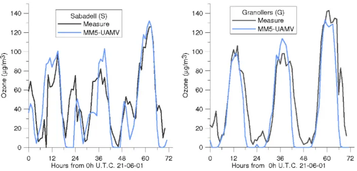
Figure 6.Hourly ozone measurement (black) and UAMV prediction (blue) for days 21, 22 and 23 of June 2001. The left panel to Granollers, and the right one corresponds to Sabadell.
results for the model were not at all sensitive to the initial conditions.
The usages of the soil were identified with those used by MM5, a 25-category database of 30” resolution from the United States Geological Survey (USGS), i.e. each of the 25 types of MM5 was assigned to one of the 11 categories recognised by UAMV. This was done from the description of each category and from the roughness.
Figure 5 shows the model output for two different times. Figure 5 (left panel) represents the spatial distribution of ozone on the early morning of 22 June, when the sun radiation was weak and there was little formation of ozone. The predominant ozone concentrations were less than 80 µg m−3 and in some near contours areas they were less than 20µg m−3. Those low levels of ozone are related to night destruction mainly due to titration effects and to low incoming radiation during morning hours. Figure 5 (right panel) represents the spatial distribution of ozone concentrations at 15 UTC. At this time the advection of air by the incoming sea breeze loaded with ozone precursors leads to high ozone concentrations. We can see the influence of the southern emissions in the central zone, which is rural and poorly habited. Note the major area of ozone concentration in dark in the centre-left of the domain. This area has no measurement station, so we must be careful with this result. This area contains forested high mountain ranges, which emit large quantities of isoprens, and is strongly influencef05d by industrial emissions, so these high ozone concentrations are possible. To control and validate the results provided by the model in this area, an experimental campaign of measurements and some ground measurement stations should be required.
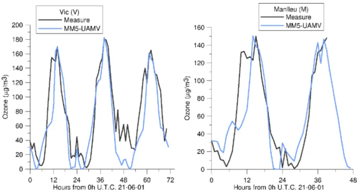
Figure 6, 7 and 8 compare the 3-day series of modelled ozone concentrations by UAMV with those observed at the six monitoring stations inside the domain. Concentrations on the lowest level of the model, which is approximately 25 m, are compared with the ambient data. These figures show the graphical validation of the MM5-UAMV performance for 72 hours, except for the Manlleu station (M), where, due to several problems, data were only available for the first 40 hours (figure 8). Qualitatively, the model simulates the ozone patterns reasonably well, particularly at the Granollers (G) station (figure 6). The low night values at the St. Celoni (C) (figure 7) and Granollers (G) (figure 6) stations were simulated well, as well as the strong increment between the night time minimum and the day time peak. However, at Sta. Maria de Palautordera (T) (figure 7), the model overpredicted the night time minimum ozone concentration, perhaps because of the rural nature of the station and the lack of precursors at night time. In the day time, the model simulated the peak ozone concentrations quite accurately, especially in Vic (V) and Manlleu (M) (figure 8). As there are often high ozone values at these stations, this was one of the main goals of the simulation. Most of the stations in this study are closer to the boundary than those at Vic (V) and Manlleu (M) and, although the peak ozone concentrations were not simulated so accurately, we considered the slight mismatch in peak ozone concentrations to be quite normal in current models. A larger domain may reduce the influence of the contour on these cells.
Figure 7.Hourly ozone measurement (black) and UAMV prediction (blue) for days 21, 22 and 23 of June 2001. The left panel corresponds to Sta. Maria de Palau Tordera, and the right one to St. Celoni.
Table 3.Statistics results for MM5-UAMV performance MM5-UAMV Mean Bias (µg m−3) -13.2 Relative Mean Bias (%) -20.7 Mean Gross Error (µg m−3) 23.8 Relative MEan Gross Error (%) 36.6 Bias for maximums (µg m−3) 1.78 Average Station Peak Normalized Bias (%) 2.0 Accuracy for maximum (µg m−3) 7.23 Average Station Peak Normalized Error (%) 5.6
ozone concentration. This underestimation may be due to the low values estimated by the model at nightime, since the model estimates the peak ozone concentration well. We can see in table 1 that the statistics related to the maximum concentration bias are small and positive. When the relative mean gross error was compared in other simulations e.g. in Jiang et al. (1998), a value of 34.8% was assigned to the CALGRID model and a value of 36.9% was assigned to the UAMV model in a four-day simulation. In our simulation, relative mean gross error was 36.6% for MM5-UAMV, which is the order of magnitude of the other two modelling systems. Our results were very good when we analysed the agreement of the peak ozone concentrations. An average station peak normalized error of 5.6% improved the results from these other simulations.
6 Models comparison
Model comparison could be done in La Plana as is the area where both models have been applied, more specifically in the Vic (V) area. A side from its own conceptual differ-ences, the models present some peculiarities.
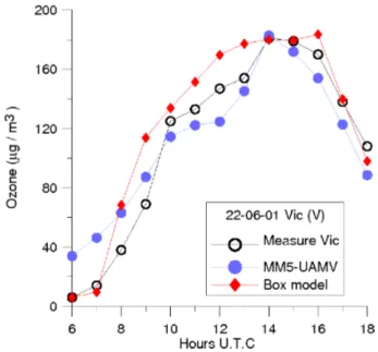
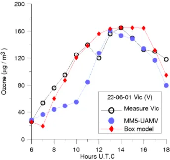
The box model has been widely used as a forecasting tool, therefore has been improved by slight modifications and is now a model that represents real ozone concentra-tions. The grid model, on the other hand, is in its first stage of development and needs more work and more simulations to become an effective tool that provides accurate and re-liable forecasts of ozone concentration. However, we have made a preliminary comparison. Figure 9, 10 and 11 show the daily ozone values predicted by both models and ozone measurements in Vic (V). Both models reproduced the ozone peak for the three days. However, the box model adjusted the measurements better during most of the daytime hours, while the grid model had a similar agreement only for 22 June. These discrepancies may be due to the fact that the box model has been specifically adjusted for the Vic area, while the grid model represents the spatial distribution of ozone concentration in a larger domain, so it is more difficult to ob-tain an accurate diurnal concentration pattern. In addition to the graphical comparison, we have calculated some statistics for each model but, as the periods evaluated are different, the results may not be representative enough. In any case, we
Figure 9.Graphical comparison of ozone from measurement sta-tion (black), UAMV simulasta-tion (blue) and box model forecast (red), in Vic on 21st of June 2001.
Figure 10.Graphical comparison of ozone from measurement sta-tion (black), UAMV simulasta-tion (blue) and box model forecast (red), in Vic on 22nd of June 2001.
Figure 11.Graphical comparison of ozone from measurement sta-tion (black), UAMV simulasta-tion (blue) and box model forecast (red), in Vic on 23rd of June 2001.
7 Conclusions
The aim of this paper was to apply two models over different areas characterized by a complex orography and affected by the presence of nearby industrial areas in which the sea breeze advects ozone and precursors to produce high ozone levels.
We analyzed the performances of a box model and a grid model in this area during different periods.
The box model was applied during the summer of 2001 in a nonoperative way but it was used in the summers of 2003 and 2004 as a forecasting tool. This helped to adjust the model specifically for different areas and the results over this longer period are quite satisfactory. Daily application of this model has shown that the main sources of error are indetermination in the emission model and in the height of the box model, but mainly in the cloudiness fraction, which is not accurately forecasted by the meteorological model.
The grid model was used during an ozone episode on three days of the summer of 2001. Although this model is only in its first stage of development, our results demonstrate its capability as its performance was good over the area we studied. Grid models take into account a wider area and can therefore forecast ozone concentrations in several locations. This requires control and quantification in order to assess the scale of ozone impacts and develop control strategies. Although the performance of the model was tested for only a short period, we found that it was highly sensitive to boundary conditions and only slightly sensitive to initial conditions. We therefore made a great effort to adjust the model’s boundary conditions, especially those regarding hydrocarbon speciation. We believe the performance of the model would improve if a larger domain were used. This would reduce the boundary effects because La Plana area would not be so close. Another way to improve performance
is to execute a nested simulation. This would require a great effort because a vast domain would have to be modelled. However, the model would be more operative because the boundary conditions for the inner domain (which would include La Plana) would come from this vast domain.
The comparison of the two models for the episode days showed good agreement between them and the measurement station. Although the box model reproduce the daily ozone behaviour better than the grid model, both maximum values are really close to the peak ozone measured.
To conclude, we should stress that we validated and compared the whole modelling systems, not just the photochemical models. The modelling system includes the meteorological model, the emission system and the photochemical model. In this way, we have demonstrated two systems with sufficient accuracy for predicting ozone concentrations.
Acknowledgements. The forecasting project was supported by the Environmental Department of the Catalan Government and by the Spanish Government through the project REN2003-03436/CLI. The authors are grateful to the very competent help of the Environ-mental Department technicians.
References
Alarc´on, M. and Alonso, S., 2001: Computing 3-D atmospheric trajectories for complex orography: application to a case study of strong convection in the western Mediterranea, Computers & Geosciences,27, 583–596.
Alarc´on, M., Alonso, S., and Cruzado, A., 1995:Atmospheric tra-jectory models for simulation of long-range transport and diffu-sion over the Western Mediterranean, Journal of Environmental Sciences and Health,A30, 1973–1994.
Berman, S., Ku, J. Y., Zhang, J., and Trivikrama, R., 1997: Uncer-tainties in estimating the mixing depth - Comparing three mixing depth models with profiler measurements, Atmospheric Environ-ment,31, 3023–3039.
Biswas, J., Hogrefe, C., Rao, S. T., Hao, W., and Sistla, G., 2001:Evaluating the performance of regional-scale photochem-ical modeling systems. Part III-Precursor predictions, Atmo-spheric Environment,35, 6129–6149.
Blackadar, A. K., 1976: Modelling the nocturnal boundary layer, Third Symposium on Atmospheric Turbulence, Diffusion and Air Quality, Raleigh, NC, Oct 19-22, American Meteorological Society, pp. 46–49.
Blackadar, A. K., 1979: Modelling pollutant transfer during day-time convection, Fourth Symposium on Atmospheric Turbulence, Diffusion and Air Quality, Reno, NV, Jan 15-18, American Me-teorological Society, pp. 443–447.
Chalita, S., Hauglustaine, D., LeTreut, H., and Muller, J.-F., 1996: Radiative forcing due to increased tropospheric ozone concen-trations, Atmospheric Environment,30, 1641–1646.
Cobourn, W. G. and Hubbard, M. C., 1999: An enhanced ozone forecasting model using air mass trajectory analysis, Bulletin American Meteorological Society,82, 945–964.
(North-eastern Spain) with a Nested Numerical Model, Meteorology and Atmospheric Physics,62, 9–22.
Dudhia, J., Gill, D., Guo, Y. R., Manning, K., Wang, W., and Chiszar, J., 2000: PSU/NCAR Mesoscale Modeling Sys-tem Tutorial Class Notes and User’s Guide: MM5 Model-ing System Version 3, National Center for Atmospheric Re-search, http://www.mmm.ucar.edu/mm5/documents/MM5\
tut\Web\notes/TutTOC.html, 138 pp.
EMEP/CORINAIR, 1999: EMEP/CORINAIR Emission Inventory Guidebook,3rd edition.
EPA, 1999: Guideline for developing an ozone forecasting pro-gram, Office of Air Quality Planning and Standards. Research Triangle Park, N.C.,EPA-254/R-99-009.
Finlayson-Pitts, B. J. and Pitts, J. N., 2000:Chemistry of the upper and lower atmosphere, Academic Press.
Gery, M., Whitten, G. Z., Killus, J. P., and Dodge, M. C., 1989: A photochemical kinematics mechanism for urban and regional scale computer modeling, Journal Geophysical Research, 94, 925–946.
Gery, M. W. and Crouse, R. R., 1990: User’s Guide for Executing OZIPR, U.S. Environmental Protection Agency, Research Trian-gle Park, N.C., EPA-9D2196NASA.
Grell, G. A., Dudhia, J., and Stauffer, D. R., 1994:A description of the fifth-generation Penn State/NCAR Mesoscale Model (MM5), NCAR/TN-398+STR. NCAR technical Note.
Grossi, P., Thunis, P., Martilli, A., and Clappier, A., 2000: Effect of sea breeze on air pollution in the greather Athens area: Part II: Analysis of different Emissions Scenarios, Journal of Applied Meteorology,39, 563–575.
Guderian, R., Tingey, D. T., and Rabe, R., 1985: Effects of photo-chemical oxidants on plants in Air Pollution by Photophoto-chemical Oxidants (edited by Guderian R.), Springer, Berlin, pp. pp. 129– 333.
Hewit, C., Lucas, P., Wellburn, A., and Fall, R., 1990:Chemistry of ozone damage to plants, Chemistry and Industry,15, 478–481. Hogrefe, C., Rao, S. T., Kasibhatla, P., Kallos, G., Tremback, C. J.,
Hao, W., Olerud, D., Xiu, A., McHenry, J., and Alapaty, K., 2001:Evaluating the performance of regional-scale photochem-ical modelling systems: Part I- metorologphotochem-ical predictions, Atmo-spheric Environment,35, 4159–4174.
Jiang, W., Hedley, M., and Singleton, D., 1998: comparison of the MC2/CALGRID and SAIMM/UAM-V photochemical mod-elling systems in the lower fraser valley, British Columbia, At-mospheric Environment,32, 2969–2980.
Kaplan, M. L., Zack, J. W., Wong, V. C., and Tuccillo, J. J., 1982: Initial results from a mesoscale atmospheric simulation system and comparisons with an AVE-SESAME I data set, Monthly Weather Review,110, 1564–1590.
Ligocki, M. P. and Whitten, G. Z., 1992: Modelling of Air Tox-ics with the Urban Airshed model, Air and Waste Management Association 85th Annual Meeting and Exhibition, Kansas City, Missouri, pp. paper 92–84.12.
Ligocki, M. P., Schulhof, R. R., Jackson, R. E., Jimenez, M. M., Whitten, G. Z., Wilson, G. M., Myers, T. C., and Fieber, J. L., 1992: Modelling the Effects of Reformulated Gasoline on Ozone and Toxics Concentration in Baltimore and Houston Ar-eas,SYSAPP-92/127.
Lippmann, M., 1991:Health effects of tropospheric ozone, Environ. Sci. Technol.,25.
McCree, K. J., 1972: Test of current definitions of photosyntheti-cally active radiation against leaf photosynthetiphotosyntheti-cally active
ra-diation against lead photosynthesis data, Agricultural Meteorol-ogy,10, 442–453.
of Catalonia, S. I., 2000:Anuari Estad´ıstic, 2000.
of Public Works of the Spanish Government, M., 2000: Monthly traffic statistics. (Estad´ıstica mensual de tr´a fico, 2000.). of Territorial Policy, D. and of Spain, P. W., 2000:Monthly Traffic
Statistics, 2000.
Pierce, T., Geron, C., Bender, L., Dennis, R., Tonnesen, G., and Guenter, A., 1998: Influence of isoprene emissions on regional ozone modeling, Journal of Geophysical Research,103, 25 611– 25 629.
Sagebiel, J. C., Zielinska, B., Pierson, W. R., and Gertler, A. W., 1996: Real-world emissions and calculated reactivities of or-ganic species from motor vehicles, Atmospheric Environment, 30, 2287–2296.
Silibello, C., Calori, G., Brusasca, G., Catenacci, G., and Finzi, G., 1998: Application of a photochemical grid model to Milan metropolitana area, Atmospheric Environment,32, 2025–2038. Sistla, G., Zhou, N., and an d S. T. Rao, W. H. J. Y. K., 1996:
Ef-fects of uncertainties in meteorological inputs of Urban Airshed Model predictions and ozone control strategies, Atmospheric En-vironment,30, 2011–2025.
Soler, M. R., Hinojosa, J., Bravo, M., D.Pino, and de Arellano, J. V. G., 2003: Analizing the basic features of different complex terrain flows by means a Doppler Sodar and a numerical model: Some implications to air pollution problems, Meteorology and Atmospheric Physics,85, 141–154.
Stockwell, R. W., Middleton, P., and Chang, J. S., 1990:The sec-ond generation Regional Acid deposition model. Chemical mech-anism for regional air quality modeling, Journal of Geophysical Research,95, 16 343–16 367.
Stull, R. B., 1984a:Transilient Turbulence Theory, Part I: The Con-cept of Eddy Mixing Across Finite Distances, Journal of Atmo-spheric Science,41, 3351–3367.
Stull, R. B., 1984b: Transilient Turbulence Theory, Part II: Tur-bulence Adjustment, Journal of Atmospheric Science,41, 3368– 3379.
Stull, R. B. and Driedonks, A. G. M., 1987: Applications of the Transilient Turbulence Parameterization to Atmospheric Bound-ary Layer Simulations, Boundary-Layer Meteorology,40, 209– 239.