A framework for upscaling short-term process-level understanding to longer time scales

(1)

HESSD

9, 6203–6224, 2012

Scaling theory

W. H. Lim and M. L. Roderick

Title Page

Abstract Introduction

Conclusions References

Tables Figures

◭ ◮

Back Close

Full Screen / Esc

Printer-friendly Version Interactive Discussion

Discussion

P

a

per

|

Dis

cussion

P

a

per

|

Discussion

P

a

per

|

Discussio

n

P

a

per

|

Hydrol. Earth Syst. Sci. Discuss., 9, 6203–6224, 2012 www.hydrol-earth-syst-sci-discuss.net/9/6203/2012/ doi:10.5194/hessd-9-6203-2012

Hydrology and Earth System Sciences Discussions

This discussion paper is/has been under review for the journal Hydrology and Earth System Sciences (HESS). Please refer to the corresponding final paper in HESS if available.

A framework for upscaling short-term

process-level understanding to longer

time scales

W. H. Lim1,3and M. L. Roderick1,2,3

1

Research School of Biology, The Australian National University, Canberra, ACT 0200, Australia

2

Research School of Earth Sciences, The Australian National University, Canberra, ACT 0200, Australia

3

Australian Research Council Centre of Excellence for Climate System Science, Australia

Received: 2 May 2012 – Accepted: 2 May 2012 – Published: 15 May 2012

Correspondence to: M. L. Roderick ([email protected])

(2)

HESSD

9, 6203–6224, 2012

Scaling theory

Title Page

Tables Figures

◭ ◮

Back Close

Full Screen / Esc

Discussion

P

a

per

|

Dis

cussion

P

a

per

|

Discussion

P

a

per

|

Discussio

n

P

a

per

|

Abstract

General experience in hydrologic modelling suggests that the parameterisation of

a model could change over different time scales. As a result, hydrologists often

re-parameterise their models whenever different temporal resolutions are required. Here,

we investigate theoretical aspects of this issue in a search for the cause(s) of the need

5

for re-parameterisations. Based on Taylor series expansion, we present a mathemati-cal framework for temporal upsmathemati-caling and evaluate it using a simple experimental sys-tem. For that, we use a unique database of half-hourly pan evaporation measurements (comprising 237 days) and examine how the model parameters change for daily and

monthly integration periods. We show that the model parameters change over different

10

integration periods with changes in the covariance between the model variables. The theory presented here is general and can be used as a basis for temporal upscaling.

1 Introduction

Thirty years ago, hydrologists had a reasonable empirical knowledge of the typical rates of many basic processes like rainfall, evaporation, infiltration, etc. One of the central

15

challenges at that time was to use that knowledge to say something useful at the larger

temporal and spatial scales of typical hydrological interest, e.g., annual runofffrom an

entire catchment or river basin, flood peak estimation, etc. Thirty years on, the term “scaling-up” invokes images of bores to monitor groundwater levels, flux towers, weirs, satellite images to document the spatial variations, that are all tied together in a spatial

20

database. These tools have proved immensely useful in the scaling of site-specific measurements. However, at the same time, much less attention has been given to the theoretical side of the scaling-up problem (Bl ¨oschl and Sivapalan, 1995; McDonnell et al., 2007).

The theoretical side of the problem is dominated by a key task – the need to

cor-25

(3)

HESSD

9, 6203–6224, 2012

Scaling theory

Title Page

Tables Figures

◭ ◮

Back Close

Full Screen / Esc

Discussion

P

a

per

|

Dis

cussion

P

a

per

|

Discussion

P

a

per

|

Discussio

n

P

a

per

|

1992; Hu and Islam, 1997a,b, 1998; Roderick, 1999; Hansen and Jones, 2000; Vogel and Sankarasubramanian, 2003; Rodriguez-Iturbe et al., 2006). That problem is not unique to hydrology – many other environmental disciplines are also grappling with the same basic problem. For example, climate scientists use the term, “sub-grid variabil-ity”, to summarise two key concepts involving the calculation of space-time averages.

5

The first key concept relates to the representation of various intensive state variables (e.g., pressure, temperature, specific humidity, etc.) in climate models that typically have very large grid cells, and it is known a priori, that the intensive state variables vary spatially within a grid cell. The second issue is how to calculate the fluxes, and thereby the changes over time, when many of the underlying processes are known

10

to be non-linear. This latter issue is of fundamental importance, because ignoring the non-linearity results in biased predictions (Larson et al., 2001). To use the classical ex-ample: the natural logarithm of the average of a group of numbers does not equal the average of the natural logarithms of the same group of numbers (Welsh et al., 1988).

The difference between those two estimates is the so-called “bias”.

15

Different approaches to handling this bias can be envisaged. The traditional

ap-proach is to use larger computers, smaller grid cells and shorter integration periods (e.g., minutes instead of hours, or hours instead of days, etc.). This is a brute-force approach, but at best, it can only reduce the bias, because to account for it completely using a numerical approach would require both infinitesimally small grid cells and time

20

periods which is not possible due to practical computing constraints. An alternative ap-proach is to account for the “bias” by directly estimating it, but to do that requires a clear theoretical understanding of what the “bias” actually is. For example, hydrologic mod-ellers are well-aware that model parameters can change with the temporal resolution

of rainfall-runoffmodels (e.g., Littlewood and Croke, 2008; Wang et al., 2009; Kavetski

25

et al., 2011) but it is difficult to clarify theoretical aspects of the “bias” using a system as

(4)

HESSD

9, 6203–6224, 2012

Scaling theory

Title Page

Tables Figures

◭ ◮

Back Close

Full Screen / Esc

Discussion

P

a

per

|

Dis

cussion

P

a

per

|

Discussion

P

a

per

|

Discussio

n

P

a

per

|

In this paper we use a unique half-hourly database of high quality pan evaporation measurements (Lim et al., 2012) to examine bias in the model predictions as a function of the model integration period. To do that we examine how the parameters of the vapour transfer function change when integrating from half-hourly to daily or monthly time periods.

5

2 Statement of the problem

Dalton’s equation for evaporation from a wet surface is,

E∝(es(Ts)−ea(Ta)) (1)

whereE (m s−1) is the evaporation rate of liquid water in traditional hydrologic units of

depth per unit time,es(Ts) (Pa) is the vapour pressure at the evaporating surface,ea(Ta)

10

(Pa) is the air vapour pressure at the same height that air temperature is measured at.

The scaling of Eq. (1) over a given period (0 toτ) can be written as

1

τ

Z

0

E dt∝1

τ

Z

0

(es(Ts)−ea(Ta)) dt

E(τ)=f_v(τ)(es(Ts)−ea(Ta)) (2)

15

wherefv(τ) (m s− 1

Pa−1) is the so-called aerodynamic function. The numerical value

of f_v(τ) generally depends on the integration period τ. In that sense, f_v(τ) can be

called an effective parameter (McNaughton, 1994). It is effective in the sense that it

will give the correct estimate ofE(τ) because it is calculated from observations using

E(τ)/(es(Ts)−ea(Ta)). That procedure means that if the time period of the model was

20

(5)

HESSD

9, 6203–6224, 2012

Scaling theory

Title Page

Tables Figures

◭ ◮

Back Close

Full Screen / Esc

Discussion

P

a

per

|

Dis

cussion

P

a

per

|

Discussion

P

a

per

|

Discussio

n

P

a

per

|

The correct scaling procedure is to begin with the full equation,

E=f_v(es(Ts)−ea(Ta))

1

τ

Z

0

E dt=1_τ τ

Z

0

f_v(es(Ts)−ea(Ta)) dt

E=fv(es(Ts)−ea(Ta)) (3)

5

wheref_v (m s−1Pa−1) is the aerodynamic function that is independent of the integration

period. By inspection we see that the correct procedure is to calculate the mean of the

product (Eq. 3) and not the product of the means (Eq. 2). To investigate the di_fferences

between Eqs. (2) and (3), we examine the scaling from short-term (e.g., half-hourly) to long-term integration periods (e.g., daily, monthly).

10

3 Theory

Based on Taylor series expansion, the theory of integrating the product of two variables

(e.g.,z=ab) over a given time period (0 toτ) can be expressed as (see Appendix A

for formal derivation)

z=ab 15

1

τ

Z

0

z dt=1_τ τ

Z

0

abdt

z=ab

=a b+σ_ab

=a b+r_[a,b]σ_aσ_b (4)

(6)

HESSD

9, 6203–6224, 2012

Scaling theory

Title Page

Tables Figures

◭ ◮

Back Close

Full Screen / Esc

Discussion

P

a

per

|

Dis

cussion

P

a

per

|

Discussion

P

a

per

|

Discussio

n

P

a

per

|

where σ_ab is the covariance between a and b, r_[a,b] (range: −1.0 to 1.0) is the

cor-relation between a and b,σa is the population standard deviation of a and σb is the

population standard deviation ofb. Note that this result is independent of the

distribu-tion of the variables. Ifr[a,b]→0 thenσab→0 and thereforeab→a b. In other words,

when the variables are uncorrelated, the mean of the product is equal to the product of

5

the means.

In the more general circumstance, the variables are correlated. We can simplify

Eq. (4) by incorporating the coefficient of variation for both aand b (i.e.,C_a≡σa

a and

Cb≡ σb

b),

z=a b(1+r[a,b]CaCb)

10

=a b(1+χ_[a,b]) (5)

whereχ_[a,b] is a correction factor arising from the covariance between a and b.

Ap-plication of Eq. (5) for a product involving more than two variables is demonstrated in Sect. 4.

15

4 Model system

Following our previous study (Lim et al., 2012), we formulate pan evaporation Epan

(m s−1) as

Epan=fv(es(Ts)−ea(Ta))

= Mw

Rρw

Dv

Ta

(es(Ts)−ea(Ta))

∆z (6)

20

wherefv (m s−

1

Pa−1) is the aerodynamic function,Mw(kg mol

−1

) is the molecular mass

of water,R (J mol−1K−1) is the ideal gas constant, ρw (kg m

−3

(7)

HESSD

9, 6203–6224, 2012

Scaling theory

Title Page Abstract Introduction Conclusions References Tables Figures ◭ ◮ ◭ ◮ Back Close

Full Screen / Esc

Printer-friendly Version Interactive Discussion Discussion P a per | Dis cussion P a per | Discussion P a per | Discussio n P a per |

water, Dv (m

2

s−1) is the diffusion coefficient for water vapour in air, Ta (K) is the air

temperature,∆z is the boundary layer thickness. In our original research, Eq. (6) was

parameterised using half-hourly data. Accordingly, we assume the resulting

param-eters to be effectively instantaneous (these parameters have been tested and found

applicable up to 6-hourly integration periods).

5

Following Eq. (3), scaling of Eq. (6) over longer term periods with constants (Mw,R)

and near-constant (ρw) removed outside the integration, we have,

E_pan= Mw

Rρw

_D

v

Ta

(es(Ts)−ea(Ta)) ∆z

(7)

Following Eq. (5), we rearrange Eq. (7) as a product of the means, Epan∗ ≡

M_w Rρ_w Dv T1_a

1

∆z (es(Ts)−ea(Ta)) that is multiplied by a collection of additive terms that are

10

associated with covariance-based correction factors. In general, for a product involving five variables, there will be ten covariance-based correction factors. In this instance,

there is one less because es(Ts) and ea(Ta) are related by a sum (and the mean of

a sum equals the sum of the means) and not a product. Using these nine covariance-based correction factors, we have,

15

Epan≃Epan∗

"

1+χh

Dv,T1a i+χ

[Dv,_∆1z]+χ[T1a, 1

∆z]+χ[Dv,es(Ts)]

es(Ts)

es(Ts)−ea(Ta)

+χ_[D_v_,e_a_(T_a)]

"

−ea(Ta)

es(Ts)−ea(Ta)

#

+χh₁

Ta,es(Ts) i

es(Ts)

es(Ts)−ea(Ta) +χh₁

Ta,ea(Ta) i

"

−ea(Ta)

es(Ts)−ea(Ta)

#

+χ_[1

∆z,es(Ts)]

es(Ts)

e_s(T_s)−e_a(T_a)

+χ_[1

∆z,ea(Ta)]

"

−ea(Ta)

e_s(T_s)−e_a(T_a) ##

(8)

20

(8)

HESSD

9, 6203–6224, 2012

Scaling theory

Title Page

Tables Figures

◭ ◮

Back Close

Full Screen / Esc

Discussion

P

a

per

|

Dis

cussion

P

a

per

|

Discussion

P

a

per

|

Discussio

n

P

a

per

|

5 Data

We use high quality (half-hourly) data collected over 237 days (during 2007–2010) at Canberra, Australia (see details in Lim et al., 2012) for evaluating the magnitude of the covariance-based corrections per Eq. (8). The daily data are aggregated into months (minimum of 16 days to be considered valid). The resulting 11 months included all

sea-5

sons (2 months in spring, 3 months in summer, 3 months in autumn and 3 months in winter).

6 Evaluating the scaling corrections

6.1 Scaling from instantaneous to daily

The magnitude of the nine covariance-based correction factors (per Eq. 8) when scaling

10

from half-hourly to a daily basis are shown in Fig. 1. We found that most (seven out

of nine) of the covariance-based correction factors (i.e.,χ) to be approximately zero

(Fig. 1a–g). The main reason for the near zero covariance-based correction factors in

seven instances is that the coefficient of variation of two variables (Dv and _T1

a) is close to zero (results not shown). In contrast, the covariance-based correction factors for the

15

remaining two terms involving the inverse of the boundary layer thickness (_∆1_z) and the

two vapour pressures (es(Ts),ea(Ta)) were relatively large (Fig. 1h, i). Physically, that

makes intuitive sense because we observed a strong diurnal variation where the wind

speed tended to increase each afternoon thereby increasing _∆1_z (Lim et al., 2012) and

resulting in a correlation between these variables.

20

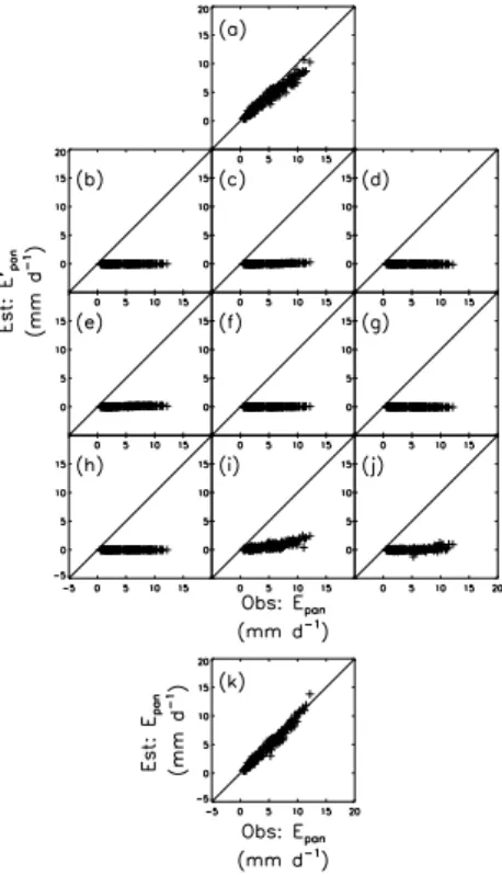
To evaluate the contribution of each covariance-based correction terms to the overall evaporation rate from the pan we plot the partial results (Fig. 2). The results confirmed an underestimate of around 20 % for the daily integrated evaporation rate when the correction terms are ignored (Fig. 2a). Only those corrections involving the inverse

of the boundary layer thickness (_∆1_z) and the two vapour pressures (es(Ts), ea(Ta))

(9)

HESSD

9, 6203–6224, 2012

Scaling theory

Title Page

Tables Figures

◭ ◮

Back Close

Full Screen / Esc

Discussion

P

a

per

|

Dis

cussion

P

a

per

|

Discussion

P

a

per

|

Discussio

n

P

a

per

|

made any significant difference to the integration (Fig. 2i, j). With those correction terms

the final results showed excellent agreement with observations (Fig. 2k, R2=0.97,

n=237, RMSE=0.50 mm d−1).

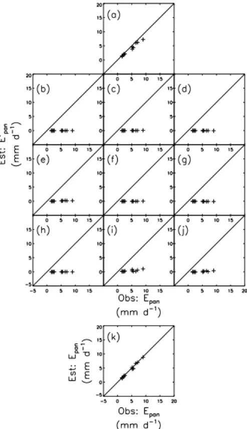
6.2 Scaling from instantaneous to monthly

We repeated the above analysis but this time we integrated from half-hourly to

5

a monthly period. The results were virtually identical with the earlier analysis based on integration to a daily time period (Fig. 3). Again, only those covariance-based

cor-rection factors involving the inverse of the boundary layer thickness (_∆1_z) with the two

vapour pressures (es(Ts), ea(Ta)) were of practical importance (Fig. 3h, i). If all the

covariance-based correction terms were ignored, the bias would result in an

underes-10

timate of monthly pan evaporation of around 17 % (Fig. 4a). Including these correction

terms gave excellent agreement with the intergated observations (Fig. 4k,R2=0.99,

n=11, RMSE=0.32 mm d−1).

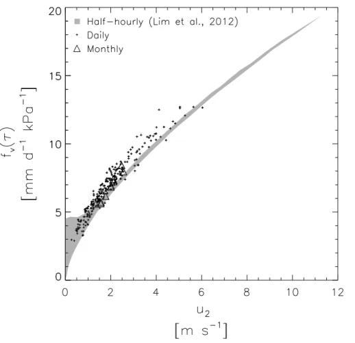
6.3 Comparing half-hourly, daily and monthly aerodynamic functions

The previous results have demonstrated that in our application, most of the

covariance-15

based correction factors make little practical di_fference. Retaining the two important

correction factorsχ that relate the inverse of the boundary layer thickness (_∆1_z) (which

increases with the wind speed) with the two vapour pressures (es(Ts),ea(Ta)), we can

rewrite Eq. (8) as

Epan≈Epan∗

"

1+χ_[1 ∆z,es(Ts)]

es(Ts)

es(Ts)−ea(Ta) +χ_[1

∆z,ea(Ta)]

"

−ea(Ta)

es(Ts)−ea(Ta)

##

(9)

20

This approximation allows us to express the aerodynamic functionfv(τ) for long-term

pan evaporation measurements from Eq. (2) in terms of the product of the means,

(10)

HESSD

9, 6203–6224, 2012

Scaling theory

Title Page

Tables Figures

◭ ◮

Back Close

Full Screen / Esc

Discussion

P

a

per

|

Dis

cussion

P

a

per

|

Discussion

P

a

per

|

Discussio

n

P

a

per

|

f_v(τ)≈f_v∗

"

1+χ_[1 ∆z,es(Ts)]

es(Ts)

es(Ts)−ea(Ta) +χ_[1

∆z,ea(Ta)]

"

−ea(Ta)

es(Ts)−ea(Ta)

##

(10)

wheref_v∗≡ Mw

Rρ_w Dv _T1

a

1

∆z. We use that expression to calculate the numerical values of

fv∗ at daily (n=237) and monthly (n=11) integration periods and compare those with

the original half-hourly results reported by Lim et al. (2012). As anticipated, the

long-5

term (daily, monthly) aerodynamic functions are generally (but not always) numerically larger than the half-hourly values because of the previously noted correlations between (_∆1_z) withes(Ts) andea(Ta) (Fig. 5).

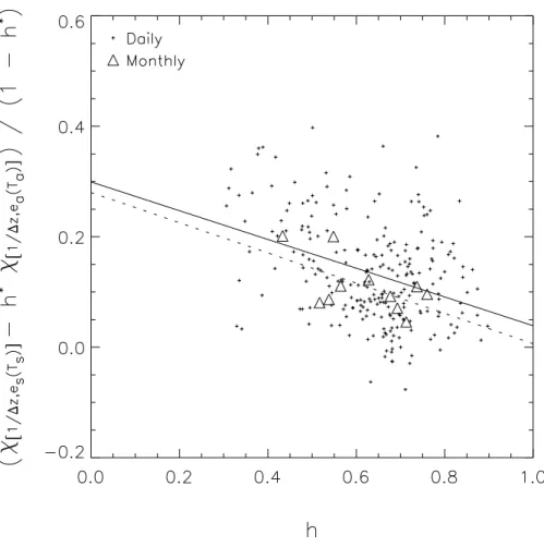
6.4 Further insights

If short-term data were available it would be straightfoward to numerically estimate

10

the two key covariance-based correction factors (i.e., χ[1

∆z,es(Ts)], χ[_∆1z,ea(Ta)]). Without doing that, one could ask whether these correction factors are themselves correlated? If so, one could make further simplifications and possibly avoid the need for detailed calculations. We found that there was no relationship between them at either daily or monthly integration periods (Fig. 6). An alternative approach is to seek a physically

15

justified relationship between these correction factors and a key environmental variable.

By defining a new variable,h∗≡ea(Ta)

e_s(T_s) we can rewrite Eq. (9) as,

Epan=Epan∗

"

1+

χ_[1

∆z,es(Ts)]−h ∗_χ

[1 ∆z,ea(Ta)] 1−h∗

#

(11)

and Eq. (10) as

f_v(τ)=f_v∗

"

1+

χ_[1

∆z,es(Ts)]−h ∗

χ_[1 ∆z,ea(Ta)] 1−h∗

#

(12)

(11)

HESSD

9, 6203–6224, 2012

Scaling theory

Title Page

Tables Figures

◭ ◮

Back Close

Full Screen / Esc

Discussion

P

a

per

|

Dis

cussion

P

a

per

|

Discussion

P

a

per

|

Discussio

n

P

a

per

|

We note that es(Ts) is not normally observed in standard operational practice.

Ac-cordingly, we compare the resulting scaling correction

χ

[1 ∆z,es(Ts)]−

h∗χ

[1 ∆z,ea(Ta)]

1−h∗ with the

observed relative humidityh

≡ea(Ta)

e_s(T_a)

over both daily and monthy integration periods

(Fig. 7). Over daily integration periods, the resulting scaling corrections varied from

−10 % to 40 % with a mean of∼13 %. Over monthly integration periods, the resulting

5

scaling corrections vary from 0 to 20 % with a mean of∼11 %. The overall (but weak)

relation to emerge is that the resulting scaling correction approaches zero when the rel-ative humidity approaches saturation (100 %). At the other extreme, when the relrel-ative humidity approaches 30 %, the resulting scaling correction approaches 25 %.

In summary, the magnitude of the scaling correction relative to the product of the

10

means (i.e.,Epan∗ ,fv∗) remain substantial and there does not appear to be a simple way

of accurately estimating that as a function of a readily measured environmental variable (e.g., relative humidity).

7 Discussion and summary

The model system used here, i.e., a half-hourly database of high quality pan

evap-15

oration measurements, is simpler than the problems typically faced in hydrology, e.g., catchment-scale water balances, etc. By using a simple system we were able to deduce deeper level insights about temporal scaling. In particular, assume an instantaneous physical relationship is accurately known as was the case here for pan evaporation. We

showed that the model parameters change for different integration periods because the

20

(12)

HESSD

9, 6203–6224, 2012

Scaling theory

Title Page

Tables Figures

◭ ◮

Back Close

Full Screen / Esc

Discussion

P

a

per

|

Dis

cussion

P

a

per

|

Discussion

P

a

per

|

Discussio

n

P

a

per

|

We followed the above-noted approach using our pan evaporation database and showed that not all covariance-based correction terms actually matter. In our example, there were nine covariance-based correction terms, yet only two of those made any

numerical difference to the results. The key physical factor in both was the inverse of

the boundary layer thickness (_∆1_z) (which increases with the wind speed). The two

im-5

portant covariance-based correction terms arose from the covariance between (i) _∆1_z

and the vapour pressure at the evaporating surfacees(Ts) and (ii)_∆1_z and the air vapour

pressureea(Ta). With those two correction terms we showed that at this site, the

nu-merical value of the aerodynamic function was generally (but not always) larger at both daily and monthly integration periods compared to the original half-hourly data (Fig. 5).

10

That arose because of a strong diurnal cycle in the pan evaporation data where the wind speed usually peaks in the mid-afternoon each day (Lim et al., 2012).

We found that the resulting scaling correction in the pan evaporation application could be readily understood as a function of the relative humidity (Fig. 7). However, that

relation was not sufficiently accurate for routine practical applications. In that sense, the

15

only alternative is to calculate the covariance-based correction using data and theory. More generally, if we were to handle the question of (temporal) scaling rigorously then we would need to begin reporting the covariances. For example, one regularly sees climatic summaries of averages yet the covariance(s) (or the variance(s) for that matter) are rarely reported. Historically, the use of manual instruments made the

re-20

(13)

HESSD

9, 6203–6224, 2012

Scaling theory

Title Page Abstract Introduction Conclusions References Tables Figures ◭ ◮ ◭ ◮ Back Close

Full Screen / Esc

Printer-friendly Version Interactive Discussion Discussion P a per | Dis cussion P a per | Discussion P a per | Discussio n P a per | Appendix A

Taylor series expansion for a product of two variables

Letzi =aibi (for i =1. . .n) be a product of two variables. We now examine the mean

z=ab by applying a Taylor series expansion in two variables (see any calculus text,

e.g., Adams, 1991) about the point (a,b) to expresszin terms ofaandb:

5

z=_n1 n

X

i=1

z_i

=_n1 n

X

i=1

z(a,b)₊1

n

X

i=1

(ai−a)

∂z ∂ai +

(bi−b)

∂z ∂bi

+_n1 n

X

i=1

1 2

"

(ai−a)2

∂2z ∂a2 i

+(ai−a)(bi−b)

∂2z ∂ai∂bi +

(bi−b)2

∂2z ∂b2 i

#

+higher order derivatives (A1)

10

where all derivatives are evaluated at (a,b). Note that, _∂a∂z

i|(a,b)=b, ∂z

∂bi|(a,b)=a, ∂2z

∂a2 i

|_(a,b)=0, ∂2z

∂b2 i

|_(a,b)=0, _∂a∂2z

ibi|(a,b)=1, and that all higher order derivatives are zero. Further, we also have,

1

n

X

i=1

(ai−a)=

1

n

X

i=1

ai−

na

a =a−a=0 (A2)

and similarly, 15 1 n n X

i=1

(14)

HESSD

9, 6203–6224, 2012

Scaling theory

Title Page

Tables Figures

◭ ◮

Back Close

Full Screen / Esc

Discussion

P

a

per

|

Dis

cussion

P

a

per

|

Discussion

P

a

per

|

Discussio

n

P

a

per

|

Thus, Eq. (A1) becomes,

z=a b=a b+1

2(0+2σab+0)=a b+σab (A4)

whereσ_ab is the covariance between variablesaandb. Note that the covariance term

emerges from the mathematics of the Taylor series expansion, and thus this result is

5

independent of the underlying distributions ofaandb.

Acknowledgements. We thank Belinda Barnes and Stephen Roxburgh who contributed ideas for earlier work on this topic. We acknowledge the Australian Research Council (ARC) for the financial support of this study through the grants DP0879763 and CE11E0098.

References 10

Adams, R. A.: Calculus: A Complete Course, Addison-Wesley, Reading, MA, 1991. 6215 Bl ¨oschl, G. and Sivapalan, M.: Scale issues in hydrological modelling: a review, Hydrol.

Pro-cess., 9, 251–290, doi:10.1002/hyp.3360090305, 1995. 6204

Hansen, J. W. and Jones, J. W.: Scaling-up crop models for climate variability applications, Agr. Syst., 65, 43–72, doi:10.1016/S0308-521X(00)00025-1, 2000. 6205

15

Hu, Z. L. and Islam, S.: Effects of spatial variability on the scaling of land surface parameteri-zations, Bound.-Lay. Meteorol., 83, 441–461, doi:10.1023/A:1000367018581, 1997a. 6205 Hu, Z. L. and Islam, S.: A framework for analyzing and designing scale invariant remote sensing

algorithms, IEEE T. Geosci. Remote, 35, 747–755, doi:10.1109/36.581996, 1997b. 6205 Hu, Z. L. and Islam, S.: Effects of subgrid-scale heterogeneity of soil wetness and tem-20

perature on grid-scale evaporation and its parametrization, Int. J. Climatol., 18, 49–63, doi:10.1002/(SICI)1097-0088(199801)18:1<49::AID-JOC224>3.0.CO;2-U, 1998. 6205 Kavetski, D., Fenicia, F., and Clark, M. P.: Impact of temporal data resolution on parameter

infer-ence and model identification in conceptual hydrological modeling: insights from an exper-imental catchment, Water Resour. Res., 47, W05501, doi:10.1029/2010WR009525, 2011. 25

6205

(15)

mod-HESSD

9, 6203–6224, 2012

Scaling theory

Title Page

Tables Figures

◭ ◮

Back Close

Full Screen / Esc

Discussion

P

a

per

|

Dis

cussion

P

a

per

|

Discussion

P

a

per

|

Discussio

n

P

a

per

|

els that ignore subgrid-scale variability, J. Atmos. Sci., 58, 1117–1128, doi:10.1175/1520-0469(2001)058<1117:sbitma>2.0.co;2, 2001. 6205

Littlewood, I. G. and Croke, B. F. W.: Data time-step dependency of conceptual rainfall-streamflow model parameters: an empirical study with implications for regionalisation, Hy-drol. Sci. J., 53, 685–695, doi:10.1623/hysj.53.4.685, 2008. 6205

5

Lim, W. H., Roderick, M. L., Hobbins, M. T., Wong, S. C., Groeneveld, P. J., Sun, F., and Farquhar, G. D.: The aerodynamics of pan evaporation, Agr. Forest Meteorol., 152, 31–43, doi:10.1016/j.agrformet.2011.08.006, 2012. 6206, 6208, 6210, 6212, 6214

McDonnell, J. J., Sivapalan, M., Vache, K., Dunn, S., Grant, G., Haggerty, R., Hinz, C., Hooper, R., Kirchner, J., Roderick, M. L., Selker, J., and Weiler, M.: Moving beyond het-10

erogeneity and process complexity: a new vision for watershed hydrology, Water Resour. Res., 43, W07301, doi:10.1029/2006WR005467, 2007. 6204

McNaughton, K. G.: E_ffective stomatal and boundary-layer resistances of heterogeneous sur-faces, Plant Cell Environ., 17, 1061–1068, doi:10.1111/j.1365-3040.1994.tb02029.x, 1994. 6206

15

Milly, P. C. D. and Eagleson, P. S.: Effects of spatial variability on annual average water balance, Water Resour. Res., 23, 2135–2143, doi:10.1029/WR023i011p02135, 1987. 6204

Rastetter, E. B., King, A. W., Cosby, B. J., Hornberger, G. M., Oneill, R. V., and Hobbie, J. E.: Ag-gregating fine-scale ecological knowledge to model coarser-scale attributes of ecosystems, Ecol. Appl., 2, 55–70, 1992. 6204

20

Roderick, M. L.: Estimating the diffuse component from daily and monthly measurements of global radiation, Agr. Forest Meteorol., 95, 169–185, doi:10.1016/S0168-1923(99)00028-3, 1999. 6205

Rodriguez-Iturbe, I., Isham, V., Cox, D. R., Manfreda, S., and Porporato, A.: Space-time model-ing of soil moisture: stochastic rainfall forcmodel-ing with heterogeneous vegetation, Water Resour. 25

Res., 42, W06D05, doi:10.1029/2005WR004497, 2006. 6205

Vogel, R. M. and Sankarasubramanian, A.: Validation of a watershed model without calibration, Water Resour. Res., 39, 1292, doi:10.1029/2002WR001940, 2003. 6205

Wang, Y., He, B., and Takase, K.: E_ffects of temporal resolution on hydrological model pa-rameters and its impact on prediction of river discharge, Hydrol. Sci. J., 54, 886–898, 30

doi:10.1623/hysj.54.5.886, 2009. 6205

(16)

HESSD

9, 6203–6224, 2012

Scaling theory

Title Page

Tables Figures

◭ ◮

Back Close

Full Screen / Esc

Discussion

P

a

per

|

Dis

cussion

P

a

per

|

Discussion

P

a

per

|

Discussio

n

P

a

per

|

Fig. 1.Relation between the covariance-based correction factors (per Eq. 8) and the relevant product of the means for all nine combination for 237 days as follows:(a)Dv, _T1_a, (b) Dv, _∆1_z, (c) 1

Ta,

1

∆z,(d)Dv,es(Ts),(e)Dv,ea(Ta),(f) T1a,es(Ts),(g)

1

Ta,ea(Ta),(h)

1

∆z,es(Ts),(g) T1a,ea(Ta),

(h) 1

(17)

HESSD

9, 6203–6224, 2012

Scaling theory

Title Page

Tables Figures

◭ ◮

Back Close

Full Screen / Esc

Discussion

P

a

per

|

Dis

cussion

P

a

per

|

Discussion

P

a

per

|

Discussio

n

P

a

per

|

Fig. 2.EstimatedE_pan(Eq. 8; prime symbol (′) denotes partial results) versus observedE_panfor

237 days:(a)E_pan∗ ,(b)χ_[_D

v,T1a]

E_pan∗ ,(c)χ_[_D

v,∆1z]E

∗

pan,(d)χ[1

Ta, 1

∆z]E

∗

pan,(e)χ[Dv,es(Ts)]

es(Ts) es(Ts)−ea(Ta)

E_pan∗ ,

(f)χ_[_D

v,ea(Ta)]

−ea(Ta) es(Ts)−ea(Ta)

E_pan∗ , (g)χ_[1

Ta,es(Ts)]

E_pan∗ ,(h) χ_[1

Ta,ea(Ta)]

E_pan∗ ,

(i)χ_[1

∆z,es(Ts)]

E_pan∗ ,(j)χ_[1

∆z,ea(Ta)]

E_pan∗ ,(k)sum of(a)to (j)(Regression:

(18)

HESSD

9, 6203–6224, 2012

Scaling theory

Title Page

Tables Figures

◭ ◮

Back Close

Full Screen / Esc

Discussion

P

a

per

|

Dis

cussion

P

a

per

|

Discussion

P

a

per

|

Discussio

n

P

a

per

|

Fig. 3.Relation between the covariance-based correction factors (per Eq. 8) and the relevant product of the means for all nine combination for 11 months as follows:(a) D_v, _T1

a,(b)Dv,

1

∆z,

(c) _T1

a,

1

∆z,(d)Dv,es(Ts),(e)Dv,ea(Ta),(f) T1a,es(Ts),(g)

1

Ta,ea(Ta),(h)

1

∆z,es(Ts),(g) T1a,ea(Ta),

(19)

HESSD

9, 6203–6224, 2012

Scaling theory

Title Page

Tables Figures

◭ ◮

Back Close

Full Screen / Esc

Discussion

P

a

per

|

Dis

cussion

P

a

per

|

Discussion

P

a

per

|

Discussio

n

P

a

per

|

Fig. 4. Estimated E_pan (Eq. 8; prime symbol (′) denotes partial results) versus ob-served E_pan for 11 months: (a) E_pan∗ , (b) χ_[_D

v,T1a]

E_pan∗ , (c) χ_[_D

v,∆1z] E

∗

pan, (d) χ[1

Ta, 1

∆z] E

∗

pan,

(e) χ_[_D

v,es(Ts)]

E_pan∗ , (f) χ_[_D

v,ea(Ta)]

E_pan∗ , (g) χ_[1

Ta,es(Ts)]

E_pan∗ ,

(h)χ_[1

Ta,ea(Ta)]

E_pan∗ , (i) χ_[1

∆z,es(Ts)]

E_pan∗ , (j) χ_[1

∆z,ea(Ta)]

E_pan∗ ,

(20)

HESSD

9, 6203–6224, 2012

Scaling theory

Title Page

Tables Figures

◭ ◮

Back Close

Full Screen / Esc

Discussion

P

a

per

|

Dis

cussion

P

a

per

|

Discussion

P

a

per

|

Discussio

n

P

a

per

|

(21)

HESSD

9, 6203–6224, 2012

Scaling theory

Title Page

Tables Figures

◭ ◮

Back Close

Full Screen / Esc

Discussion

P

a

per

|

Dis

cussion

P

a

per

|

Discussion

P

a

per

|

Discussio

n

P

a

per

|

(22)

HESSD

9, 6203–6224, 2012

Scaling theory

Title Page

Tables Figures

◭ ◮

Back Close

Full Screen / Esc

Discussion

P

a

per

|

Dis

cussion

P

a

per

|

Discussion

P

a

per

|

Discussio

n

P

a

per

|