Abstract
The prediction of plastic instability in sheet metals during forming processes represents nowadays an ambitious challenge. To reach this goal, a new numerical approach, based on the loss of ellipticity criterion, is proposed in the present contribution. A polycrystalline model is implemented as a user-material subroutine into the ABAQUS/Implicit finite element (FE) code. The polycrystalline constitutive model is assigned to each integration point of the FE mesh. To derive the mechanical behavior of this polycrystalline aggregate from the behavior of its microscopic constituents, the multiscale self-consistent scheme is used. The mechanical behavior of the single crystals is described by a finite strain rate-independent constitutive framework, where the Schmid law is used to model the plastic flow. The condition of loss of ellipticity at the macroscale is used as plastic instability criterion in the FE model-ing. This numerical approach, which couples the FE method with the self-consistent scheme, is used to simulate a deep drawing process, and the above criterion is used to predict the formability limit of the studied sheets during this operation.
Keywords
crystal plasticity, loss of ellipticity, self-consistent, finite elements, forming limit diagrams
Prediction of Plastic Instability in Sheet Metals During
Forming Processes Using the Loss of Ellipticity Approach
1 INTRODUCTION
For weight reduction of automotive parts, there is nowadays a growing need for designing new lightweight high strength metallic materials (Heller et al., 1998). To meet this industrial demand, these new materials should present some desirable in-use properties, such as high strength and im-proved ductility. They are generally characterized by their strong anisotropy, which is the most important physical phenomenon that affects the strength and the formability of sheet metals (Guan et al., 2006). Considering the high costs relating to the experimental characterization of these new alloys, numerical simulation tools are expected to provide a valuable alternative to be used to assess
H.K. Akpama a, * M. Ben Bettaieb a F. Abed-Meraim a
a LEM3, UMR CNRS 7239 – Arts et
Métiers ParisTech, 4 rue Augustin Fresnel, 57078 Metz Cedex 3, France. DAMAS, Laboratory of Excellence on Design of Alloy Metals for low-mAss Structures, Université de Lorraine, France.
[email protected] [email protected] [email protected]
* Corresponding author
http://dx.doi.org/10.1590/1679-78253544
the strength and the formability of these new materials. This performance evaluation is considered to be an essential step in the strategy of the design of industrial parts produced from these materi-als (Nakamachi, 1997). In order to evaluate their formability during sheet metal forming processes, finite element (FE) analyses are frequently used in the automotive industry. However, reliable FE simulations of forming processes require an accurate description of the initial and induced anisotro-py of the studied sheet metals. Unfortunately, phenomenological approaches, which have been wide-ly used for several decades in the FE simulations, are not able to accuratewide-ly account for this initial and induced anisotropy. To overcome this limitation, various micromechanical models have been developed and incorporated into FE analyses to simulate different forming processes (Beaudoin et al., 1994; Guan et al., 2006; Nakamachi et al., 2001). The advantage of such micromechanical modeling, compared to phenomenological approaches, is its ability to link, in a natural way, several material features (initial and induced anisotropy, grain morphology…) to some important in-use properties (strength, formability …). Thanks to the substantial increase in computational power, the use of micromechanical constitutive frameworks in the simulation of complex forming processes becomes an interesting and feasible alternative to phenomenological models, the latter having been intensively used in the past.
In the present investigation, the numerical strategy based on the coupling between microme-chanical modeling and FE analysis is followed. The self-consistent approach (Lipinski and Berveil-ler, 1989) is used as multiscale scheme in this micromechanical modeling. Within this approach, each single crystal is assumed to be an ellipsoidal inclusion contained in a fictitious homogeneous medium endowed with the same mechanical features as the polycrystalline aggregate. In contrast to the Taylor model, which is more commonly used in this kind of coupled strategies (Guan et al., 2006; Jung et al., 2013), the equilibrium equations at the grain level are fully satisfied when the self-consistent approach is used. Moreover, this choice allows considering some effects that cannot be taken into account with the Taylor model, such as the impact of grain morphology. Furthermore, the Taylor model may be viewed as a particular case of the self-consistent approach. The mechani-cal behavior of the single crystals is described by a finite strain rate-independent constitutive framework, where the Schmid law is used to model the plastic flow.
single finite element in this preliminary application allows assimilating the studied medium to an infinite block of material, which is homogeneously deformed until the incipience of localization bi-furcation. Accordingly, the loss of ellipticity phenomenon can be viewed as the result of an intrinsic material instability with no structural effects. In this first application, the material instability of the studied polycrystalline aggregate has been represented through the well-known concept of forming limit diagrams (Keeler and Backofen, 1963). Then, the above-described numerical implementation has been used to simulate the deep drawing of various sheet specimens. It is noteworthy that this second application allows the evolution of microstructural properties (crystallographic texture as well as grain morphology) to be accurately predicted during deep drawing processes. In these deep drawing simulations, the loss of ellipticity phenomenon may be attributed to competing material and structural instabilities.
The reminding parts of the paper are structured as follows:
The second Section is devoted to the presentation of the constitutive frameworks both at the single crystal and polycrystal scales.
The theoretical framework for the loss of ellipticity approach is presented in the third Sec-tion.
In the fourth Section, two numerical applications mainly are shown to illustrate the efficiency of the implemented numerical strategy.
Notations, conventions and abbreviations
The notations, conventions and abbreviations used in this paper are clarified in the box bellow. Additional notations will be provided as needed.
Vector and tensor fields are designated by bold letters and symbols.
Scalar variables and parameters are represented by thin letters and symbols.
Microscopic (resp. macroscopic) variables are referenced by lowercase (resp. capital) letters.
Einstein’s convention of implied summation over repeated indices is adopted. The range of free (resp. dummy) index is given before (resp. after) the corresponding equation.
· time derivative of · 2
I the second-order identity tensor
4
I the fourth-order identity tensor
• lattice co-rotational derivative of ·
1
•- inverse of · .
· · inner product
• : • double contraction product
•Ä• tensor product
2 CONSTITUTIVE FRAMEWORKS AT THE SINGLE CRYSTAL AND POLYCRYSTAL SCALES
In this section, several developments will be carried out in order to express the behavior laws both at the single crystal and polycrystal scales in the following generic forms:
: : , single crystal behavior law (microscopic level):
polycrystal behavior law (macroscopic level): =
=
n l g
N G (1)
where:
n (resp. N ) is the microscopic (resp. macroscopic) nominal stress rate tensor.
l (resp. ) is the microscopic (resp. macroscopic) tangent modulus.
g (resp. G) is the microscopic (resp. macroscopic) velocity gradient tensor.
The aim of the following sections is to derive the explicit expressions for both the microscopic (Section 2.1) and macroscopic (Section 2.2) tangent moduli.
2.1 Single Crystal Scale
The microscopic velocity gradient g can be additively decomposed into its symmetric and
skew-symmetric parts denoted as d and w, respectively
= +
g d w
.
(2)Considering the fact that elastic deformation is sufficiently small compared to plastic defor-mation, d and w can be in turn split into their elastic and plastic parts
;
e p e p
= + = +
d d d w w w
.
(3)The rotation r of the single crystal lattice frame is determined by we and satisfies the relation
below
. T = e
r r w
.
(4)Because plastic slip occurs along specific crystallographic directions, on particular crystallo-graphic planes, the components dp and wp of the plastic part gp of the velocity gradient can be
written in the following form:
sgn( ) ; 1,..., sgn( ) p s p N
a a a
a a a
g a g
t
t
ìï = ïï = íï = ïïî d Rw P
.
(5)where:
a
g is the absolute value of the slip rate on the -th slip system.
a
R and Pa are the symmetric and skew-symmetric parts of the Schmid orientation tensor
a Ä a
a
m and na are the slip direction and the slip plane normal vector, respectively. In the single crys-tal lattice frame, the counterpart ma0 (resp. na0) of ma (resp. na) remains fixed during the de-formation. Vectors ma0 and na0 are related to ma and na by the following relations:
0 0
. ; . T
a = a a = a
m r m n n r
.
(6)s
N is the total number of slip systems.
a
t is the resolved shear stress defined as the projection of the Cauchy stress tensor s on the Schmid orientation tensor ma Äna:
: ( )
a a a
t =s m Än
.
(7)The elastic part of the behavior law classically relates the co-rotational derivative s of the
Kirchhoff stress tensor to the elastic strain rate de as follows:
:
e e
=
s d
.
(8)where e is the fourth-order elasticity tensor. Here, linear isotropic elasticity is assumed. We recall that the Kirchhoff stress tensor s is related to the Cauchy stress tensor s by the following rela-tion:
j
=
s s
,
(9)where j is the jacobian of the deformation gradient.
The relation between the time derivative s of the Kirchhoff stress tensor and its co-rotational
derivative reads
. e e.
= - +
s s s w w s
.
(10)The nominal stress tensor n is defined by the relation = j 1.
n f- s and, adopting an updated Lagrangian approach, its rate n reads
Tr( ) .
= +
-n s s d gs
.
(11)The latter can be related to the slip rates ga by combining Eqs. (3), (5), (8)-(11)
: . . ( : . . ) sgn( )
e e a a a a a
g t
= - - - +
-
n d s w d s R P s s P . (12)
The plastic flow rule used to determine the expression of the slip rates ga results from the Schmid criterion (Schmid and Boas, 1935). This criterion states that plastic slip occurs only when the absolute value of the resolved shear stress ta on slip system a reaches a critical value tca,
(
)
1,...,Ns : a ca a 0
a t t g
" = - = . (13)
The overall strain hardening characteristic of the material is modeled by the introduction of a hardening matrix h, which describes the evolution of the critical resolved shear stress tca
1,...,Ns : ca hab b ; 1,...,Ns
a t g b
" = = = . (14)
The following consistency condition can be derived from the Schmid law (13)
: asgn( a) ca 0 ; a 0
a t t t g
" Î - = > , (15)
where is the set of active slip systems. The slip rates of the slip systems that do not belong to set are obviously equal to zero.
The time derivative of the resolved shear stress ta is given by the following expression:
: ( )
a a a
t = s m Än , (16)
where s is defined by the following relation:
. e e.
= + w -w
s s s s. (17)
By using Eqs. (3) and (8), ta can be further developed as follows:
1,...,Ns : a a : e : Tr( ) sgn( b) b a : e : b ; 1,...,Ns
a t é ù t g b
" = = ê - ú- =
ë û
R d s d R R . (18)
The combination of Eqs. (14), (15) and (18) leads to the following expression for the slip rates
a
g :
(
2)
: a Jabsgn( b) b : e : ;
a g t b
" Î = R -sÄI d Î, (19)
where J is the inverse of matrix M defined by the following index form:
(
)
: sgn( )sgn( ) : :
,
b Mab hab ta b a e ba
Î = +t
"
R R . (20)By introducing relation (19) into Eq. (12), one finally obtains the following expression for the microscopic tangent modulus l:
(
)
(
(
)
)
1 2
2
sgn( )sgn( ) : . . : ; ,
e
e e
l
J
a b ab a a a b
t t a b
= -
-- + - Ä - Ä Î
l l
R P P R I
s s
s s s (21)
where the fourth-order tensors 1l
s and s2l are the terms induced by lattice rotation within the
1 1( ) ; 2 1( )
2 2
ijkl jl ik jk il ijkl ik jl il jk
l = d s -d s l = d s +d s
s s (22)
2.2 Polycrystalline Scale
The self-consistent scale-transition scheme is adopted for deriving the overall macroscopic behavior from knowledge of the behavior of individual single crystals. The main lines of the approach are recalled hereafter; the reader may refer to (Lipinski and Berveiller, 1989; Lipinski et al., 1995) for more details. The macroscopic tensor fields are defined as the volume averages of their microscopic counterparts, and they are related through fourth-order concentration tensors A and B in order to
solve the averaging problem
( ) ( ) : ; ( ) ( ) : .
g x A x G n x B x N (23)
Making use of Eqs. (1) and (23), the generic form of the macroscopic tangent modulus can be expressed as follows:
1
( ) : ( ) ( ) : ( )
V dv
V
=
ò
l x A x = l x A x . (24)
For a polycrystalline aggregate composed of ellipsoidal crystals with different crystallographic orientations, the behavior and mechanical fields of each individual grain are assumed to be homoge-neous. Denoting by gI (respectively lI) the volume average of the velocity gradient (respectively
tangent modulus) for a grain I within the polycrystalline aggregate, and using some elaborate deri-vations based on Green’s tensors (Lipinski et al., 1995), we can demonstrate that the concentration tensor AI corresponding to grain
I is given by
(
)
1(
)
1 14 : ( ) : 4 : ( )
I II I II I
--
-= - - -
-A I T l I T l , (25)
where TII is the interaction tensor for grain I , related to Eshelby’s tensor (Eshelby, 1957) for an
ellipsoidal inhomogeneity.
Furthermore, in order to simplify the integral equation, the assumption of homogeneous defor-mation inside each individual grain is made. Accordingly, if we introduce the indicator function
( )
I
q x defined as
( ) V
( ) V
I I
I I
1 if
0 if
q q
ìïïï íï ïïî
x x
x x , (26)
then
( )x = I qI( ) ; ( )= IqI( ) ; I =1,...,Ng
where VI denotes the volume of grain
I and Ng the number of grains that make up the polycrys-talline aggregate.
Under the above assumption of homogeneity of the microscopic mechanical fields, Eq. (24), which defines the macroscopic tangent modulus, can be equivalently expressed as
: ; 1,...,
I I I
g
f I N
= l A =
, (28)
where fI represents the volume fraction of grain
I .
3 LOSS OF ELLIPTICITY APPROACH
The bifurcation theory developed in Rudnicki and Rice (1975) is known to be a relevant approach for the prediction of material instabilities associated with jumps in strain rates across a localization band.
Because field equations have to be satisfied, the kinematic condition for the strain rate jump reads
= Ä
G C , (29)
where:
X is the jump of the field X across the discontinuity band. C is the jump vector.
is the unit vector normal to the localization band.
On the other hand, the continuity of the equilibrium of forces through the band is expressed as:
. = 0
N
. (30)
The combination of Eqs. (29) and (30) with the behavior law (1) leads to the following equa-tion:
.( : Ä )=0
C
, (31)
which is equivalent to
( . . ). 0
C
, (32)
det ( . . )=0 (33)
Eq. (33) is the so-called Rice bifurcation criterion (Rudnicki and Rice, 1975), which corresponds to the loss of ellipticity of the partial differential equations governing the associated boundary value problem.
4 NUMERICAL PREDICTIONS AND DISCUSSIONS
The developed polycrystalline constitutive framework and the associated loss of ellipticity criterion have been implemented into the finite element code ABAQUS/Standard as user-material (UMAT) subroutine. Various numerical simulations based on these implementations are presented in this section. After the material data used in the different simulations are specified, the implemented model is first used to predict the formability of a sheet metal in the form of forming limit diagrams. Then, a deep drawing process is simulated using the implemented model.
4.1 Material Data
In this section, the microscopic material data used to simulate the stress–strain response of poly-crystalline aggregates, on the basis of the self-consistent model, are presented. The values of the material parameters are chosen in the range of those for rolled aluminum sheets. Thus, the follow-ing choices and material parameters are adopted in the remainder of the paper:
Single crystals with FCC crystallographic structure are used in what follows. For this crystal-lographic structure, the number of slip systems Ns is equal to 12. More details on the
num-bering of the corresponding slip system vectors, m0a and n0a, can be found in Bettaieb et al.
(2012).
The Poisson ratio and the Young modulus are set to 0.33 and 67.7 GPa, respectively.
The initial critical resolved shear stress t0 is assumed to be the same for the different slip systems and is taken equal to 40 MPa.
Similar to several investigations conducted in the literature on FCC materials, an isotropic hardening matrix is used to describe the evolution of the critical resolved shear stresses inside the single crystals. Accordingly, the components hab of the hardening matrix h are taken to
be identical and equal to h. The hardening modulus h is given by the following power law: 1
0 0
0
0 0
1 ;
s
n t N
h
h h dt
n
a
a
g t
-= æ G ÷ö
ç ÷
ç
= çç + ÷÷ G =
÷
çè ø
ò
å
, (34)where n is the power-law hardening exponent and h0 is the initial hardening rate. The values of n
and h0 are set equal to 0.35 and 390 MPa, respectively.
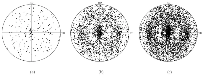
tex-tures of these different polycrystalline aggregates are randomly generated and are displayed in Fig-ure 1.
RD
TD
RD
TD
RD
TD
(a) (b) (c)
Figure 1: Initial texture of the studied polycrystalline aggregates, {111} pole figure: (a) 50 grains; (b) 500 grains; (c) 1000 grains.
The different polycrystalline aggregates (with 50, 500, and 1000 grains) are simulated by sub-jecting them to a uniaxial tension along the rolling direction. The simulated tensile stress–strain responses associated with these three polycrystalline aggregates are shown in Figure 2. It can be observed that the uniaxial tensile stress–strain responses corresponding to the polycrystals with 500 and 1000 grains are practically the same. However, the response of the polycrystal with 50 grains is relatively different from the others. These preliminary results suggest that 500 grains is a reasonable choice to be adopted in order to generate a polycrystalline aggregate that can be considered to be representative of the studied material.
0.00 0.15 0.30 0.45 0.60 0
150 300 450 600
50 grains
500 grains
1000 grains
S
11 (MPa)
E11
4.2 FLD Predictions
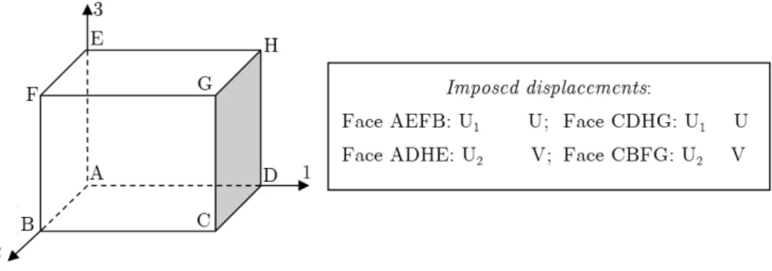
In order to numerically predict the formability of sheet metals in the form of forming limit diagrams (FLDs), a single C3D8R solid finite element is considered. As illustrated in Figure 3, displacement-type boundary conditions, which evolve over time, are prescribed to this eight-node hexahedral element. The evolution of the displacements U and V, applied to the faces CDHG and CBFG, re-spectively, are defined by the following relations:
11 11
( ) t ; ( ) t
U t =ee V t =er e , (35)
where is the strain-path ratio, assumed to be constant during the deformation to guarantee the proportionality of the strain paths. This strain-path ratio is varied in the range -1 / 2£ £r 1 to span the complete FLD. It is noteworthy that the plane stress state is a natural outcome of the prescribed boundary conditions. Indeed, as the face EFGH is free from any constraint, the stress components S13, S23, and S33 are obviously equal to 0.
Figure 3:Illustration of the boundary conditions applied to a single finite element.
Fur-thermore, it is also observed from Figure 4 that the predictions given by the polycrystalline aggre-gate with 50 grains exhibit much more oscillations than those obtained with the other polycrystal-line aggregates, which comprise a larger number of grains. Indeed, the smoothness in the simulated curves is closely related to the continuous character of the macroscopic tangent modulus, which is itself determined by the tangent moduli of the constituent grains. However, at the grain level, the tangent modulus is not smooth due to the discrete nature of the slip system activity (i.e., the set
of active slip systems introduced in Section 2.1 changes very frequently during the deformation). Consequently, a sufficiently large number of grains is required to obtain a relatively smooth evolu-tion for the minimum of the determinant of the acoustic tensor. Moreover, Figure 4 clearly shows that the simulation results given by the polycrystal with 500 grains are quite close to those predict-ed by the polycrystal with 1000 grains, especially for the strain paths r =0, 0.5, and 1. These results support once again the idea that a polycrystalline aggregate with 500 grains or more pro-vides a good representation for the mechanical behavior of the polycrystalline material.
0.0 0.2 0.4 0.6 0.8 0 1x10² 2x10² 3x10² 4x10² 5x10²
( )1/3
. .
Minéêëdet ùúû
50 grains
500 grains
1000 grains
E
11
r = -0.5
0.0 0.1 0.2 0.3 0.4 0 1x10² 2x10² 3x10² 4x10² 5x10² E11 ( )1/3
. .
Minéêëdet ùúû
50 grains
500 grains
1000 grains
r = 0
(a) (b)
0.0 0.1 0.2 0.3 0.4 0 1x10² 2x10² 3x10² 4x10² 5x10²
( )1/3
. .
Minéêëdet ùúû
50 grains
500 grains
1000 grains
E11 r = 0.5
0.0 0.1 0.2 0.3 0.4 0 1x10² 2x10² 3x10² 4x10² 5x10²
( )1/3
. .
Minéêëdet ùúû
50 grains
500 grains
1000 grains
E11 r = 1
(c) (d)
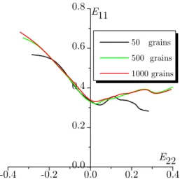
The effect of the number of grains on the shape and location of the predicted FLDs is investi-gated in Figure 5. This figure clearly reveals large differences between the FLD predicted by the polycrystalline aggregate with 50 grains and the other FLDs, especially in the range of positive strain paths. This result confirms the preliminary trends observed in Figure 5. Furthermore, plastic strain localization is predicted at realistic strain levels in the range of position strain-path ratios (r³ 0), in contrast to phenomenological flow theories with associative plasticity and smooth yield surface, which generally require the introduction of some softening phenomena, such as those in-duced by ductile damage (Mansouri et al., 2014). The realistic level for the predicted limit strains is made possible here thanks to the yield surface vertex structure (inherent in crystal plasticity theo-ry), which arises from the discrete nature of crystalline slip.
-0.4 -0.2 0.00.0 0.2 0.4
0.2 0.4 0.6 0.8
E22 E11
50 grains
500 grains
1000 grains
Figure 5: Forming limit diagrams for the different polycrystalline aggregates (50, 500, and 1000 grains).
4.3 Deep Drawing Simulations
In order to efficiently simulate the deep drawing process using the developed multiscale model, a sensitivity analysis has been carried out in order to select the optimal number of grains to be used for representing the polycrystalline aggregate associated with each macroscopic integration point of the mesh. Based on this study, it is found that an aggregate with 500 grains seems to be a pragmat-ic compromise in terms of good representativeness of the actual material and reasonable CPU times required to run the various FE simulations. The initial crystallographic texture used for all of the integration points in the various FE models studied in the current Section is the same as that pre-sented in Figure 1 (b).
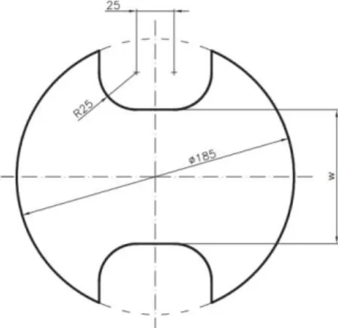
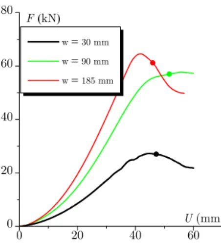
tions: 30 mm, 90 mm, and 185 mm (the latter corresponds to a circular specimen). The specimen width w is varied in order to reproduce different strain paths in the center of the specimen: the values 30 mm, 90 mm, and 185 mm correspond to uniaxial tensile state (r = -0.5), plane-stress tensile state (r = 0), and equi-biaxial tensile state (r =1), respectively. The different tools (die, punch, and blank holder) are modeled as analytical rigid surfaces, while the specimens are meshed using C3D8R linear solid finite elements. In order to capture the bending effects and hence to im-prove the computation accuracy, three layers of elements are used in the thickness direction. This choice seems to be a pragmatic compromise in terms of good accuracy of the results and reasonable computational times. The mesh density is increased in the contact zone between the punch and the specimen. To carry out the forming process, the punch is displaced in the vertical direction up to a maximal displacement of 60 mm.
Figure 6:Schematic description of the tools used in the simulation of the deep drawing process.
Figure 7:Dimensional characteristics of the circular and notched specimens used in the Nakajima tests (Kami et al., 2015).
0 20 40 60 0
20 40 60 80
w30 mm w 90 mm w185 mm
F(kN)
U (mm)
Figure 8: Punch force–displacement curves for the different specimen geometries.
Figure 9 shows the deformed shapes for the various Nakajima specimens, with the associated von Mises equivalent stress distribution, at the onset of plastic instability. One may notice that the value of equivalent stress is relatively low in the central area of the specimens. However, this von Mises equivalent stress reaches its maximal values in narrow zones near the dome apex.
(a) (b) (c)
Figure 9: Distribution of the von Mises equivalent stress in the various Nakajima specimens at the onset of plastic instability: (a) Specimen with w = 30 mm; (b) Specimen with w = 90 mm; (c) Specimen with w = 185 mm.
indi-cator takes as value 0 (resp. 1) when the minimum of the determinant of the acoustic tensor, over all possible localization band orientations, is positive (resp. negative). Red (resp. blue) color is used in Figure 10 to designate the finite elements where the loss of ellipticity indicator is equal to 1 (resp. 0). The plastic instability, which corresponds to the nullity of the loss of ellipticity indicator, is first reached in the dome apex region, where the von Mises equivalent stress is maximal (see Fig-ure 9). For more clarity, the corresponding elements in red color are surrounded by more visible red circles in Figure 10.
(a) (b) (c)
Figure 10: Distribution of the loss of ellipticity indicator in the different Nakajima specimens at the onset of plastic instability: (a) Specimen with w = 30 mm; (b) Specimen with w = 90 mm; (c) Specimen with w = 185 mm.
The distribution of the loss of ellipticity indicator in the different Nakajima specimens at the end of the simulation (punch depth = 60 mm) is shown in Figure 11. It is observed from this figure that the instability zone has extended to the entire dome apex region.
(a) (b) (c)
Figure 11: Distribution of the loss of ellipticity indicator in the different Nakajima specimens at the end of the simulation (punch depth = 60 mm): (a) Specimen with
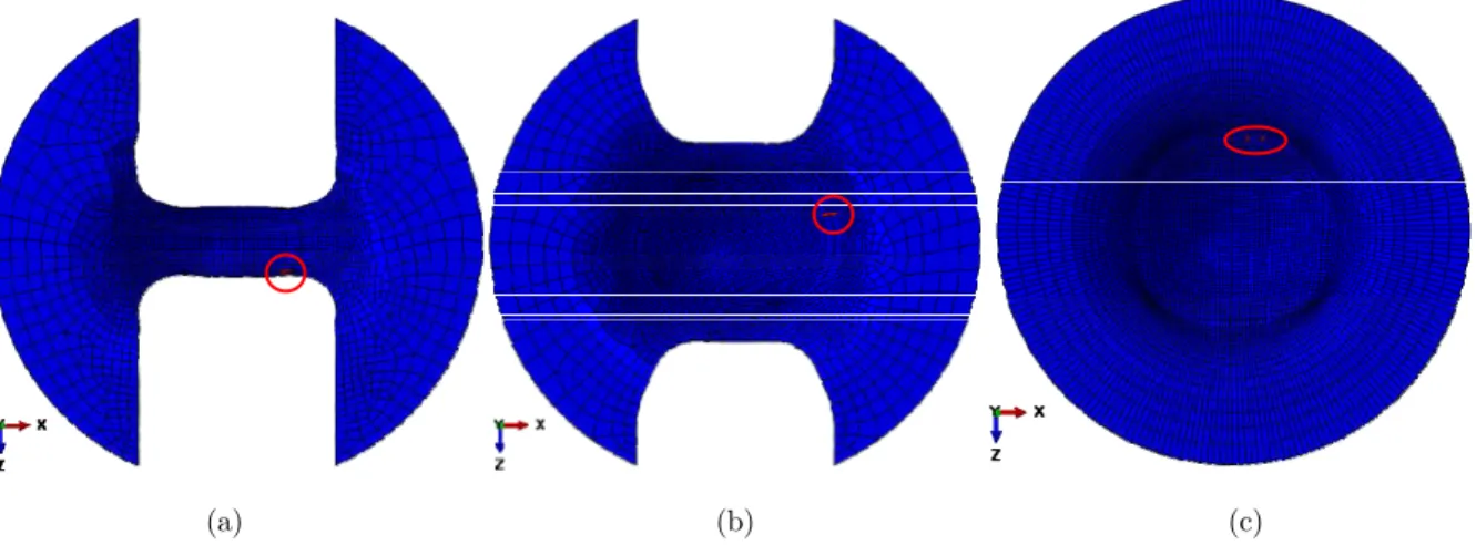
In order to better understand the initiation and evolution of the instability, three particular el-ements are selected in each specimen for the following analysis: Element A (Elem. A), which corre-sponds to the central element of the specimen, Element B (Elem. B), which is representative of the zone near the localization area, and Element C (Elem. C), which corresponds to the element where the instability is first triggered (see Figure 12).
(a) (b) (c)
Figure 12:Locations of the different analyzed elements: (a) Specimen with w = 30 mm; (b) Specimen with w = 90 mm; (c) Specimen with w = 185 mm.
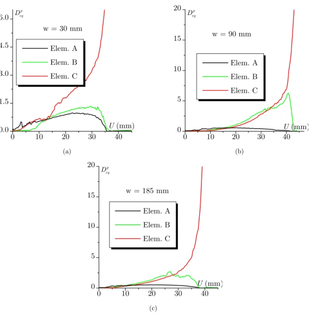
The evolution of the von Mises equivalent plastic strain rate p eq
D as a function of the punch
displacement for the different analyzed elements and the different specimens is shown in Figure 13. It is clearly observed from this figure that Elem. A (resp. Elem. C) has the lower (resp. higher) strain rate among the three analyzed elements. Consequently, Elem. A exhibits the slower defor-mation, while Elem. C displays the more rapid plastic defordefor-mation, which ultimately tends to local-ize. This trend is common to the three specimens. Note however that the different elements do not have the same evolution for p
eq
D . Indeed, for Elem. A and Elem. B, p eq
D increases before the onset of instability in the specimen, while it decreases afterwards, which typically corresponds to elastic unloading in these elements. On the other hand, p
eq
0 10 20 30 40 0.0
1.5 3.0 4.5 6.0
p eq D
Elem. A
Elem. B
Elem. C
U (mm) w = 30 mm
0 10 20 30 40
0 5 10 15
20 p
eq D
Elem. A
Elem. B
Elem. C
U (mm) w = 90 mm
(a) (b)
0 10 20 30 40
0 5 10 15
20 p
eq D
Elem. A
Elem. B
Elem. C
U (mm) w = 185 mm
(c)
Figure 13: Evolution of the equivalent plastic strain rate as a function of the punch depth U: (a) Specimen with w = 30 mm; (b) Specimen with w = 90 mm; (c) Specimen with w = 185 mm.
influ-ence of deformation-induced anisotropy due to grain rotation during plastic deformation may not be quite important at the end of the simulation. On the other hand, the final textures corresponding to Elem. C are significantly different from the initial texture shown in Figure 1 (b). This result is also quite expectable considering the significant evolution of the strain rate in this element, as observed in Figure 13.
RD
TD
RD
TD
RD
TD
(a) (b) (c)
RD
TD
RD
TD
RD
TD
(d) (e) (f)
RD
TD
RD
TD
RD
TD
(g) (h) (i)
5 CONCLUDING REMARKS
In order to accurately simulate sheet forming processes, a suitable constitutive framework is re-quired. To this aim, a multiscale polycrystalline model has been developed and implemented into the ABAQUS/Implicit finite element code. In this physically-based model, the link between the microscopic and macroscopic scales is achieved by using the self-consistent scale-transition scheme. The proposed model accounts for the initial and induced plastic anisotropy through the modeling of the texture evolution. The implemented constitutive model has been coupled with an indicator of loss of ellipticity in order to predict the occurrence of macroscopic plastic instability. This coupling has been used mainly in the following two applications:
To investigate the effect of the number of grains, which constitute the polycrystalline aggre-gate, on the predicted forming limit diagram.
To predict the onset and the evolution of plastic instability within sheet specimens undergo-ing a deep drawundergo-ing process.
References
Akpama, H. K., Ben Bettaieb, M., Abed-Meraim, F. (2016). Influence of the yield surface curvature on the forming limit diagrams predicted by crystal plasticity theory. Latin American Journal of Solids and Structures 13:2231–2250. Beaudoin, A. J., Dawson, P. R., Mathur, K. K., Kocks, U. F., Korzekwa, D. A. (1994). Application of polycrystal plasticity to sheet forming. Computer Methods in Applied Mechanics and Engineering 117:49–70.
Ben Bettaieb, M., & Abed-Meraim, F. (2015). Investigation of localized necking in substrate-supported metal layers: comparison of bifurcation and imperfection analyses. International Journal of Plasticity 65:168–190.
Ben Bettaieb, M., Débordes, O., Dogui, A., Duchêne, L., Keller, C. (2012). On the numerical integration of rate independent single crystal behavior at large strain. International Journal of Plasticity 32:184–217.
Eshelby, J. D. 1957. The determination of the elastic field of an ellipsoidal inclusion, and related problems. In Pro-ceedings of the Royal Society of London A: Mathematical, Physical and Engineering Sciences. 241:376–396.
Guan, Y., Pourboghrat, F., Barlat, F. (2006). Finite element modeling of tube hydroforming of polycrystalline alu-minum alloy extrusions. International Journal of Plasticity 22:2366–2393.
Heller, T., Engl, B., Ehrhardt, B., Esdohr, J. (1998). New high-strength steels-production, properties and applica-tions. In Iron and Steel Society/AIME, 40th Mechanical Working and Steel Processing Conference Proceedings 36:25–34.
Jung, K. H., Kim, D. K., Im, Y. T., Lee, Y. S. (2013). Prediction of the effects of hardening and texture heterogenei-ties by finite element analysis based on the Taylor model. International Journal of Plasticity 42:120–140.
Kami, A., Dariani, B. M., Vanini, A. S., Comsa, D. S., Banabic, D. (2015). Numerical determination of the forming limit curves of anisotropic sheet metals using GTN damage model. Journal of Materials Processing Technology 216:472–483.
Keeler, S. P., Backofen, W. A. (1963). Plastic instability and fracture in sheets stretched over rigid punches. Trans-actions of the ASM 56:25–48.
Lipinski, P., Berveiller, M. (1989). Elastoplasticity of micro-inhomogeneous metals at large strains. International Journal of Plasticity 5:149–172.
Lipinski, P., Berveiller, M., Reubrez, E., Morreale, J. (1995). Transition theories of elastic-plastic deformation of metallic polycrystals. Archive of Applied Mechanics 65:291–311.
Nakamachi, E. (1997). Optimum design of metal forming based on finite element analysis and nonlinear program-ming. In Tatsumi, T. et al. (Eds.), Theoretical and Applied Mechanics 1996:323–340.
Nakamachi, E., Xie, C. L., Harimoto, M. (2001). Drawability assessment of BCC steel sheet by using elas-tic/crystalline viscoplastic finite element analyses. International Journal of Mechanical Sciences 43:631–652.
Rudnicki, J. W., Rice, J. R. (1975). Conditions for the localization of deformation in pressure-sensitive dilatant mate-rials. Journal of the Mechanics and Physics of Solids 23:371–394.