ISSN 0104-6632 Printed in Brazil
www.abeq.org.br/bjche
Vol. 27, No. 03, pp. 391 - 399, July - September, 2010
Brazilian Journal
of Chemical
Engineering
ON THE PREDICTION OF PSD IN ANTISOLVENT
MEDIATED CRYSTALLIZATION PROCESSES
BASED ON FOKKER-PLANCK EQUATIONS
M. Grosso
1*, R. Baratti
1and J. A. Romagnoli
1,21Dipartimento di Ingegneria Chimica e Materiali, Università degli Studi di Cagliari,
Piazza d’Armi, I-09123, Cagliari, Italy. 2
On leave from Department of Chemical Engineering, Lousiana State University, USA E-mail: [email protected]
(Submitted: December 19, 2010 ; Revised: May 24, 2010 ; Accepted: June 22, 2010)
Abstract - A phenomenological model for the description of antisolvent mediated crystal growth processes is presented. The crystal size growth dynamics is supposed to be driven by a deterministic growth factor coupled to a stochastic component. Two different models for the stochastic component are investigated: a Linear and a Geometric Brownian motion terms. The evolution in time of the particle size distribution is then described in terms of the Fokker-Planck equation. Validations against experimental data are presented for the NaCl-water-ethanol anti-solvent crystallization system. It was found that a proper modeling of the stochastic component does have an impact on the model capabilities to fit the experimental data. In particular, the GBM assumption is better suited to describe the antisolvent crystal growth process under examination.
Keywords: Antisolvent crystallization; Particle size distribution estimation; Fokker-Planck equation.
INTRODUCTION
Antisolvent aided crystallization is a technique widely used in solid-liquid separation processes. In this method, a secondary solvent known as the antisolvent or precipitant is added to the solution, resulting in the reduction of the solubility of the solute, and supersaturation is then induced. The trend of supersaturation generation during the process has a direct and significant role on crystal characteristics such as size, morphology and purity. In this regard, control of the size distribution is a crucial point of interest for the application and several factors can affect the broadening of the size distribution.
To this end, the development of effective mathematical models describing the crystal growth dynamics is a crucial issue and can be a useful tool to find the optimal process performance. The main approach exploited so far is by developing population balance (PB) models (e.g., Ramkrishna, 2000), taking
into account the evolution of crystal particles across temporal and size domains. This method implies first principle assumptions, requiring a detailed knowledge of the physics and thermodynamics of the process. Some important contributions to this subject have been reported in the literature (e.g., Worlitschek and Mazzotti, 2004; Bakir et al, 2006; Nowee et al., 2008; Nagy et al, 2008). However, they demand a great deal of knowledge of the complex thermodynamic associated with the solute and solvent properties to be adequately incorporated in the population balances. Thus, a disadvantage could be that the resulting model would be too complex to be employed, for example, for model-based process control design.
motion, whereas the deterministic contribution (the so-called drift term) was assumed to follow a logistic equation. Under these conditions the state variable is no longer a deterministic variable, but is a random one, whose probability density can be described in terms of the Fokker-Planck equation (FPE). The main advantage of this approach is its simplicity: it requires only a model that qualitatively describe the process behavior, without the necessity of a deep physical-chemical knowledge. On the other hand, traditional PB approaches involve a detailed formulation and estimation of the corresponding parameters of the particular kinetic mechanism involved in the crystallization process.
A quantitative agreement between experimental observations and the model was eventually observed and the approach seems to be promising for exploitation for particle size control policies in order to determine the optimal antisolvent feed rates strategies. In this stochastic formulation, however, the modeling of the random motion was found to be a crucial task for the model performance: the assumption of a specific Brownian motion implies that diffusion coefficients may indeed affect deeply the shape of the Particle Size Distribution.
In the present work, we investigated the performance capabilities of two different stochastic models to describe experimental data provided by the NaCl-water-ethanol anti-solvent crystallization system. The PSD was measured at different time instants using a Mastersizer 2000 particle size analyzer. Two different models are considered here, which differ by the diffusion term: (i) a traditional linear diffusive term related to a constant linear Brownian motion, (ii) a nonlinear one related to Geometric Brownian Motion. Model calibration was carried out for different antisolvent feed rates. It was eventually assessed that a nonlinear Geometric Brownian motion is preferable to predict quantitatively the log-normal shape of the experimental data. Such analysis further confirms the assumptions made in a previous contribution (Grosso et al., 2010).
The Mathematical Models
The crystals are classified by their size, L, the growth of each individual crystal is assumed to be independent of the other crystals and governed by the same deterministic model. In the proposed model, fluctuations and unknown dynamics not captured by the deterministic term are modeled as a random component that has an additive action on the growth dynamics (Gelb, 1988).
( ) ( )
( )
dL
g L t Lf L, t
dt = Γ + (1)
where L is the random variable describing the time evolution of the crystal size, Γ(t) is the Langevin force:
( )
t 0Γ = (2)
( ) ( )
t t ' 2(
t t ')
Γ Γ = δ − (3)
and the term Lf(L,t) is the deterministic contribution associated with the crystal growth. By applying the Stratanovich approach in a one-dimensional space, one eventually ends up with the Fokker-Planck equation describing the dynamical equation for the probability density ψ(L,t) given in Equation (4) (Risken, 1984; Fa, 2005):
( )
( )
( ) ( )
( ) ( )
L, tg L g L L, t
t L L
L, t Lf L, t L
∂ψ = ∂ ⎛ ∂ ⎡ ψ ⎤⎞−
⎜ ⎣ ⎦⎟
∂ ∂ ⎝ ∂ ⎠
∂ ψ ∂
(4)
The choice of the specific form for g(L) leads to different shapes for the probability density function. In the present contribution, we investigate the performance of FPEs based on different expressions for g(L).
1. Linear Brownian Motion (LBM) Model
As a first option, a constant value g(L) = 2 D is assumed
( )
( )
dL
2 D t L f L, t L 0
dt = Γ + > (5)
One should note that: i) when the deterministic drift term f = 0, Equation (5) describes the classical Wiener process; ii) when f is constant, Equation (5) describes an Ornstein-Uhlenbeck process. In both cases, the random variable L follows a Gaussian distribution. Equation (5) can be manipulated in order to obtain the Langevin equation for the random variable y = lnL:
( ) ( )
1 dL 2 D
t f L, t L 0
that is:
( )
y( )
dy
2 D t e h y
dt
−
= Γ + (7)
where L = exp(y), and h(y) is a deterministic model to be chosen. The FPE for the new random variable y can be eventually rewritten as:
( )
( ) ( )
2 2y2
y, t
D e 3 2y
t y y
y, t h y y
− ⎛ ⎞
∂ψ = ∂ ψ− ∂ψ+ −
⎜ ⎟
⎜ ⎟
∂ ⎝∂ ∂ ⎠
∂ ψ ∂
(8)
2. Geometric Brownian Motion (GBM) Model
Conversely, assuming a linear dependence on the crystal size L, g(L) = 2 D L, Equation (1) can be rewritten as
( )
( )
dL
2 DL t L f L, t L 0
dt = Γ + > (9)
When f is constant, Equation (9) describes a Geometric Brownian Motion (GBM). It should be noted that, when the GBM assumption holds, the associated PDF is a log normal distribution (Ross, 2003). If f also depends on L, some distortions from the ideal log normal case can, however, be expected. This feature is qualitatively observed for many (although not all) crystalline substances (Eberl et al, 1990). Manipulating Equation (9), one can eventually obtain the Langevin equation for the random variable y = lnL
( ) ( )
dy2 D t h L, t
dt = Γ + (10)
and the corresponding FPE is:
( )
2( ) ( )
2
y, t
D y, t h y
t y y
∂ψ = ∂ ψ− ∂ ψ
∂ ∂ ∂ (11)
It should be noted that, when h = 0, the actual FPE is the typical diffusive equation for the Brownian motion, whose solution is a Gaussian distribution for the y variable (thus a log normal distribution for the L variable).
As regards the deterministic part of the model, a Logistic growth process is here assumed (cf.,
Tsoularis and Wallace, 2002).
( )
yh y r y 1 K
⎛ ⎞
= ⎜ − ⎟
⎝ ⎠ (12)
This choice is mainly motivated to the requirement for a simple model with a parsimonious number of adjustable parameters, i.e., the growth rate, r, and the asymptotic equilibrium value K. The present growth model can be regarded as a phenomenological model providing, in a qualitative fashion, the main features of a generic growth process: the growth follows a linear law with slope given by r at low crystal size values and saturates at a higher equilibrium value K.
Regardless of the stochastic model to be adopted, the boundary conditions considered are the same, that is:
( )
y, t0, y , t
y
∂ψ
= → −∞ ∀
∂ (13)
( )
y, t0, y , t
y
∂ψ
= → +∞ ∀
∂ (14)
which ensure that the ψ(y,t) PDF preserves its integral on the space domain, i.e. the normality assumption is always assured.
EXPERIMENTS AND METHODS
Crystal size [mm] 100
ψ
(
L
)
0.0 0.4 0.8
t
Crystal size [mm]
0 100 200 300 400 500
ψ
(
L
)
0.0 0.4 0.8
t = 34 min t = 56 min t = 114 min t = 197 min t = 240 min
t
(a) (b)
Figure 1: Experimental PSD from the Mastersizer particle size analyzer for the low antisolvent feed rate u0 = 1.5 ml/min at different sampling times during the batch (Figure 1a: logarithmic scale; Figure 1b: linear scale)
Model calibration for the estimation of parameters is carried out separately for every run. The parameters to be estimated are: θ = [log(D), r, K] (log(D) is used instead of D in order to reduce the statistic correlation between the parameters). It should be noted that direct measurements of the Particle Size Distribution are available at N different spatial locations and at M different time values for every operating condition, i.e., anti-solvent flow rate. Parameter inference is accomplished by using the least square criterion, thus searching for the minimum of the objective function:
( )
(
)
(
)
(
)
(
)
m n
2
mod k j exp k j
j 1 k 1
r, K, D
y , t y , t
= =
Φ θ = Φ =
ψ θ − ψ
∑∑
(15)
In Equation (15), ψmod(yk,tj) is the probability density function evaluated through numerical integration of Equations (8) or (11), depending on the model selected, at time tj and size coordinate yk, while the distribution ψexp(yk,tj) is the experimental observation of the PSD for the size coordinate yk at time ti. The parameter inference is thus carried out by comparing N point observations of the distribution (N ~ 40), monitored at M different times (M between 6 and 10, depending on the experimental run). The minimum search is performed by exploiting the Levenberg-Marquardt method.
The performance of the model calibration is carried out by evaluating the Mean Square Error s2, defined here as:
(
)
(
)
(
)
( )
m n
2 mod k j exp k j j 1 k 1
2
y , t y , t
ˆ s
m n m n
= =
ψ θ − ψ
Φ θ
= =
⋅ ⋅
∑∑
(16)
In Equation (16), ˆθis the vector of parameter values which minimize the objective function.
Comparison between model and experiments is also accomplished by reporting the time evolution of the experimental observations and the corresponding model prediction for first moments of the distribution, i.e., the mean, μ and the variance σ2:
( )
0L L dL
∞
μ =
∫
ψ (17)
(
) ( )
22 0
L L dL
∞
σ =
∫
− μ ψ (18)RESULTS
The point estimation values for the model parameters, together with the related Mean Square Errors s2, are reported in Table 1.
diffusive term is supposed to affect the shape of the probability distribution and, conversely, it should not affect the deterministic part of the process. It was instead found that the dependence of the parameter estimation on the diffusive term is appreciable. This aspect will be further discussed later.
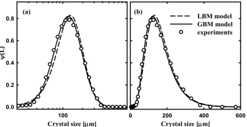
Figure 2 and Figure 3 report some results related to the comparison of the experimental PSD with the model predictions for the GBM model (solid line) and the LBM model (dashed line). The data refer to
the feed rate u0 = 1.63 ml min-1 at an intermediate time t= 58.63 min (Figure 2) and at t = 120 min, i.e., the final time of the experimental run (Figure 3). Similar results are, however, observed even at the other feed rates and times. The crystal size is shown on both logarithmic (Figures a) and linear scales (Figures b). It appears that both the models are able to capture the main features of the experimental PSD. However, the FPE-GBM model evidently outperforms the FPE=LBM model in all cases.
Table 1: Estimated parameters for the different operating conditions for the LBM and GBM models with the related s2
Feed flow (ml/min) r K log10(D) s2
0.83 8.353e-4 7.667 0.3757 2.68e-3 1.65 1.460e-3 7.678 0.3545 8.981e-4
( )
g L = D
(LBM) 3.2 2.077e-3 7.678 0.3556 9.965e-4
0.83 1.788e-2 4.8779 -2.402 7.96e-4
1.65 1.800e-2 4.8640 -2.391 2.84e-4
( )
g L = DL
(GBM) 3.2 8.475e-2 4.6781 -1.702 4.09e-4
L [μm]
200 400 600
L [μm]
10 100 1000
ψ
(L)
0.0 0.2 0.4 0.6 0.8 1.0
GBM model LBM model Experiments
(a) (b)
Figure 2: Comparison between model and the experimental PSD for the antisolvent feed rate u0=1.63 ml min-1 at t=58.63 min. Solid line is the GBM model, dashed line is the LBM model, white circles are the experimental observations. Figure (a): the crystal size is on a logarithmic scale; Figure (b): the crystal size is on a decimal scale.
Crystal size [μm]
0 200 400 600
Crystal size [μm] 100
ψ
(
L
)
0.0 0.2 0.4 0.6
0.8 LBM model
GBM model experiments
(a) (b)
Figure 3: Comparison between model and the experimental PSD for the antisolvent feed rate u0=1.63 ml min -1
More insight into the descriptive characteristics of the alternative models can be obtained by analyzing the time evolution of the experimental observations and the corresponding model prediction for first moments of the distribution, i.e., the mean μ, and the variance σ2. Figures 4 and 5 show, respectively, the mean and variance experimentally observed (square points) compared with the theoretical predictions for the three runs as a function of time, for the GBM model (solid line) and the LBM model (dashed line). It is remarkable that the dynamic behavior of the two models is quite different. The GBM model almost reaches the asymptotic equilibrium value at the end of the
experimental run. Conversely, the LBM model appears to be far from the equilibrium solution, a feature that is clearly in contrast with the experimental evidence and the physical situation.
From the previous results, it is clear that the GBM stochastic model, driven by its deterministic part (the logistic growth term), correctly describes the increasing trend of the average crystal growth and the asymptotic behavior. In Figures 4b and 5b, we also report experimental data provided by the second experimental run (cross points), (not used for the parameter inference), here used for an a posteriori validation. They demonstrate that the GBM model also has good predictive capabilities.
time [min]
10 20 30 40 50 60 70
time [min]
20 40 60 80 100 120 140
time [min]
50 100 150 200 250
μexp
, μ
mo
d
[μ
m
]
100 110 120 130 140 150
GB Model LB Model Experiments
(a) (b) (c)
Figure 4: Mean of the Crystal Size Distributions for the three feed rates Square points are the experimental observations, solid lines are the GBM model predictions, dashed lines are the LBM model predictions. Cross points in Figure b are additional experimental data not used for the parameter inference.
time [min]
10 20 30 40 50 60 70
time [min]
50 100 150 200 250
σ
2 mod
,
σ
2 ex
p
[
μ
m
2]
2000 3000 4000 5000 6000
Experiments LBM model GBM model
time [min]
20 40 60 80 100 120
(a) (b) (c)
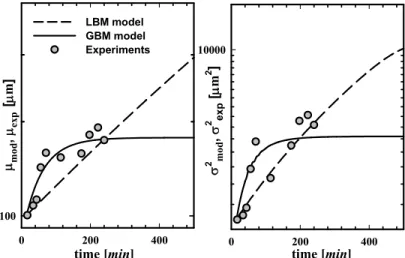
Finally, as a further analysis for the model comparison, the time evolution of the mean and the variance of the crystal size distributions are reported for the two models in Figure 5 over a time window much larger than the one used for the experiments. The purpose of the analysis is to appreciate the long-time dynamics and check their capabilities to reasonably describe the asymptotic behavior. Both LBM and GBM models are integrated at the parameter values inferred by the parameter estimation at u0=3.2 ml/min. For the sake of completeness, the experimental values are also reported. Keeping in mind that the r parameter gives a measurement of the characteristic process time, it is clear that the transient time in the LBM model (the order of magnitude is τ = 1/r ~ 103) is clearly overestimated with respect to the one obtained with
the GBM model (where τ = 1/r ~ 101÷102). The latter characteristic time is more likely to describe the experimental evidence of the process under consideration. As a final remark, for these parameter conditions, the steady state regime is shown to be experimentally reached after a rather short transient period (~ 200 min).
These differences between the models are further evidenced in Figure 7, where the long-time evolution of the PSD for the LBM and GBM models at low flow rates are reported. It is clearly shown that the LBM model has not yet reached the equilibrium regime solution after 500 minutes, whereas the GBM model appears constant for t > 200 min. This result further confirms that the GBM model is more suited to correctly capture the process dynamics of the crystal growth process.
time [min]
0 200 400
μmod
, μ
exp
[μ
m
]
100
time [min]
0 200 400
σ
2 mod
,
σ
2 exp
[
μ
m
2 ]
10000 LBM model
GBM model Experiments
Figure 6: Long-time evolution of mean and variance for the LBM model (dashed line) and the GBM model (solid line). The model parameters used are related to high feed rate conditions. Circles are the experimental points.
crystal size [μm]
ti
me [min]
102
50 100 150 200 250 300 350 400 450
crystal size [μm]
ti
me [min]
102
50 100 150 200 250 300 350 400 450
CONCLUSIONS
A phenomenological stochastic model for the description of antisolvent crystal growth processes was presented. In this formulation, the crystal size was considered as a random variable, whose probability density evolution in time could be described in terms of a Fokker-Planck equation. Furthermore, a comparative assessment of the predictive capabilities of the model under alternative models for the stochastic component was carried out. From the study, it was found and corroborated by experimental data that the nonlinear Geometric Brownian motion is preferable to quantitatively predict the log-normal shape of the experimental data.
The models were tested on data provided by a bench-scale fed-batch crystallization unit where anti-solvent is added to speed-up the crystal formation process. The FPE-GBM formulation is found to be a powerful predictive tool, as confirmed by the excellent agreement with the experiments.
ACKNOWLEDGMENTS
Jose Romagnoli kindly acknowledges the Regione Sardegna for the support through the program “Visiting Professor 2009”.
Massimiliano Grosso acknowledges PRIN-2006091953 project for its financial support.
NOMENCLATURE
D FPE pseudo-diffusivity term min-1 K Equilibrium value logistic
model
(-)
f deterministic function on a linear scale
g noise function
h deterministic function on a logarithmic scale
L Crystal size μm
m number of experiments n number of experimental
points for the experimental PSD
r Growth rate logistic model min-1
s2 Mean square error
t time Min
u0 antisolvent feed rate ml min-1
y crystal size on the logarithmic scale
(-)
Greek Letters
Γ Langevin force
θ parameters vector
μ mean of the PDF on a linear scale
μm
σ2 variance of the PDF on a linear scale
μm2
ψ probability density function (PDF)
REFERENCES
Bakir, T., Othman, S., Fevotte, G., Hammouri, H., Nonlinear observer of crystal-size distribution during batch crystallization. AIChE J., 52, 2188-2197 (2006).
Eberl, D. D., Srodon, J., Kralik, M. and Taylor, B. E., Ostwald ripening of clays and metamorphic minerals. Science, 248, 474 (1990).
Fa, K. S., Exact solution of the Fokker-Planck equation for a broad class of diffusion coefficients. Phys. Rev., E, 72, 020101(R) (2005).
Galán, O., Grosso, M., Baratti, R., Romagnoli, J., A stochastic approach for the calculation of anti-solvent addition policies in crystallization operations: An application to a bench-scale semi-batch crystallizer. Chem. Eng. Sci., 65, 1797-1810, (2010).
Gelb, A., Applied Optimal Estimator. M.I.T. Press, Cambridge (Massachusetts) (1988).
Grosso, M., Galán, O., Baratti, R., Romagnoli, J., A stochastic formulation for the description of the crystal size distribution in antisolvent crystallization processes. AIChE J., 56, (8), 2077-2087 (2010).
Nagy, Z. K., Fujiwara, M. and Braatz, R. D., Modelling and control of combined cooling and antisolvent crystallization processes. J. Proc. Cont., 18, No. 9, 856 (2008).
Ramkrishna, D., Population balances theory and
applications to particulate systems in engineering. San Diego: Academic Press (2000).
Risken, H., The Fokker-Planck Equation: Methods of Solutions and Applications. Springer-Verlag, Berlin (1996).
Ross, S. M., An Elementary Introduction to Mathematical Finance: Options and other Topics,
Cambridge University Press, Cambridge (2003). Tsoularis, A. and Wallace, J., Analysis of Logistic
Growth Models. Mathematical Biosciences, 179, 21 (2002).
Worlitschek, J. and Mazzotti, M., Model-Based Optimization of Particle Size Distribution in Batch-Cooling Crystallization of Paracetamol. Crystal Growth & Design, 4, No. 5, 891 (2004).