Braz. J. Chem. Eng. vol.27 número3

ISSN 0104-6632 Printed in Brazil

www.abeq.org.br/bjche

Vol. 27, No. 03, pp. 381 - 390, July - September, 2010

*To whom correspondence should be addressed

This is an extended version of the manuscript presented at the PSE 2009 - 10th International Symposium on Process Systems Engineering, 2009, Salvador, Brazil, and published in Computer Aided Chemical Engineering, vol. 27, p. 579-584.

Brazilian Journal

of Chemical

Engineering

A FAST AND SYSTEMATIC PROCEDURE TO

DEVELOP DYNAMIC MODELS OF

BIOPROCESSES - APPLICATION TO

MICROALGAE CULTURES

J. Mailier

1

and A. Vande Wouwer

2*

Control Department, Engineering Faculty, University of Mons (UMONS), 31 Boulevard Dolez, B-7000 Mons, Belgium.

1

Phone: +32-(0)65374133, Fax: +32-(0)065374136 E-mail: [email protected]

2

Phone: +32-(0)65374141, Fax: +32-(0)065374136 E-mail: [email protected]

(Submitted : December 11, 2009 ; Revised : May 13, 2010 ; Accepted : May 18, 2010)

Abstract - The purpose of this paper is to report on the development of a procedure for inferring black-box, yet biologically interpretable, dynamic models of bioprocesses based on sets of measurements of a few external components (biomass, substrates, and products of interest). The procedure has three main steps: (a) the determination of the number of macroscopic biological reactions linking the measured components; (b) the estimation of a first reaction scheme, which has interesting mathematical properties, but might lack a biological interpretation; and (c) the "projection" (or transformation) of this reaction scheme onto a biologically-consistent scheme. The advantage of the method is that it allows the fast prototyping of models for the culture of microorganisms that are not well documented. The good performance of the third step of the method is demonstrated by application to an example of microalgal culture.

Keywords: Reaction networks; Mathematical modeling; Parameter estimation; Bioprocesses.

INTRODUCTION

The increasing demand for process monitoring, control, and optimization encourages the development of various techniques for modeling bioprocesses. Among these techniques, the one proposed by Bastin and Dochain (1990) relies on the concept of a macroscopic reaction scheme, i.e., a set of M

reactions that represent macroscopic relationships between the N key-components of the system (biomass, substrates, and products). The general form of a macroscopic reaction scheme can be expressed as:

[

]

k

k

ik i jk j

i j

, ,

k

( ) for k 1, M

∈ ∈

−ν ξ ⎯ϕ⎯⎯→ ν ξ ∈

∑

∑

R P

(1)

where R_k and Pk are, respectively, the sets of reactants and products of reaction k , and ϕ_k is the kth reaction rate, generally expressed as a non-negative, nonlinear function of the reacting species concentrations ξ_i and ξ_j. The coefficients ν_*k are the pseudo-stoichiometric (or yield) coefficients of reaction k , which are positive when related to a product and negative for a reactant. A necessary condition for independence between the reactions is to force their number to be less than or equal to the number of components, i.e., M≤N.

essential biological aspects that are of interest for further process monitoring and optimization. Assuming for the sake of clarity no gaseous outflow, a simple mass balance thus gives the following set of ordinary differential equations, written in matrix form:

( ) ( ) ( )

d (t)

K D(t) t F t , dt

ξ _{= ϕ ξ − ξ +}

(2)

where ξ( )t ∈RN is the vector of species concentrations,K∈RM N× the pseudo-stoichiometric matrix, ϕ ξ ∈( ) RMthe reaction rate vector,

( )

D t ∈R the input dilution rate, and F t( )∈RN the vector of external feed rates. From Equation (2), it is obvious that the model reactions are linearly independent if and only if matrix K is full rank:

( ) .

rank K =M (3)

The next section introduces the three successive stages of the identification methodology and the subsequent section illustrates its use in a simulation example of microalgal growth, using a mechanistic reformulation of the well-known Droop model (Lemesle and Mailleret, 2008).

ROBUST METHODOLOGY OF IDENTIFICATION

The present work concerns the identification of model (2) from a limited set of noisy measurements of the state vector:

( )

e

m _e

e k

s

e 1, , N t , with ,

k 1, , N = … ⎧

ξ _⎨

= …

⎩ (4)

where N is the number of informative experiments e

and N is the number of samples taken during the _se eth experiment. Discrete instant t refers to the e_k kth measurement time of the eth experiment. It is assumed that the initial concentrations of all the experiments are measured with special care, so that they can be regarded as perfectly known:

( )

e ( )

m t0 0 , e.

ξ = ξ ∀ (5)

This assumption can eventually be relaxed by estimating initial conditions, together with the

unknown parameters of Equation (2). In our methodology, the distinction is made between three types of such parameters:

ƒ M , the minimum number of reactions to be * taken into account in order to represent the experimental data with a given accuracy;

ƒ ϑ*_K, the optimum stoichiometric parameters, which are the unknown elements of the yield matrix K ; and

ƒ ϑ*_ϕ, the optimum kinetic parameters appearing in the reaction rate vector ( )ϕ ξ .

It is assumed that the biological information available on the process encompasses the structure of the reaction rate vector. Also, full-state measurement is assumed at discrete times, so that a continuous, noise-reduced signal ξ_m

( )

t is obtained via standard techniques of interpolation and linear filtering. Finally, the time-evolution of the dilution rate and external feed rates are regarded as perfectly known. Number of Reactions

As described by Bernard and Bastin (2005a, 2005b), the number of reactions required for the model to reproduce the observations with a given error threshold can be assessed by a principal component analysis of the interpolated datasets. Their estimation approach is briefly outlined in what follows.

After placing the measured terms on the left-hand side of the equation, Equation (2) can be written as follows for every measurement instant:

( ) ( ) ( )

( )

( )

e

k

e e e e

k k k k

(t t )

d (t)

D t t F t K t .

dt ₌

ξ _{+ ξ − = ϕ ξ}

(6)

The interpolation and linear filtering of both sides of this expression gives

( )

( )

u t =Kw t , (7)

which can be written in matrix form after sorting column-wise the vectors related to the various instants:

U=KW. (8)

Brazilian Journal of Chemical Engineering Vol. 27, No. 03, pp. 381 - 390, July - September, 2010

T T

UU =P ΣP, (9)

where Σ is a diagonal, positive semi-definite matrix whose nonzero elements represent the variance related to each eigenvector, i.e., each column of matrix P . The first stage of the methodology thus consists of selecting the set of the M largest eigenvalues that represent a total variance larger than a given confidence threshold.

Identification of C-Identifiable Schemes

A systematic, data-driven approach was suggested by Hulhoven et al. (2005) to identify those reaction schemes that satisfy a mathematical property known as C-identifiability. This procedure relies on a state transformation operated via the following partition of the pseudo-stoichiometric matrix:

( )

M M a

a

N M M

b _b

K K

K , with .

K _K

×

− ×

⎧ _∈

⎛ ⎞ ⎪

=_{⎜ ⎟ ⎨}

⎝ ⎠ _⎪⎩ ∈

R

R (10)

The matrix C is chosen such that

a b

CK +K =0, (11)

which makes the dynamics of the transformed state vector z= ξ + ξC _{a b} independent of the reaction rate vector:

( ) ( )

a b

dz(t)

D t z t CF (t) F (t).

dt = − + + (12)

Using Equation (12), the measurement of z(t) and the knowledge of the transport terms enable the estimation of C independently of the reaction kinetics (Bogaerts et al., 2003). The property of C-identifiability denotes those schemes whose pseudo-stoichiometric matrix can be computed as the unique solution of Equation (11) when an estimate of C is known (Chen and Bastin, 1996).

The identification approach recommended by Hulhoven et al. (2005) ensures model C-identifiability by systematically screening those matrices K that have the following specific form: a

a

1 0 0

0 1

K .

0

0 0 1

± …

⎛ ⎞

⎜ _± ⎟

⎜ ⎟

=

⎜ ⎟

⎜ _{… ±} ⎟

⎝ ⎠

% #

# % % (13)

By determining the value of K that offers the a

smallest cost after identification of its corresponding matrix C , an estimate of the whole pseudo-stoichiometric matrix is deduced from Equation (11). This identification procedure is repeated for every possible partition [ξ ξ_a, _b]T of the state vector and the pseudo-stoichiometric matrix leading to the smallest cost function is eventually adopted.

The second step of our methodology makes the most of the observation that real bioprocess models are usually not C-identifiable because their submatrix K is rarely of the form (13). Rather than _a spending computational effort in screening all the possible values of K suggested by (13), which _a would lead anyway to reaction schemes lacking biological interpretation, our approach keeps K _a equal to identity the first time. Doing so speeds up the algorithm by restricting the screening of many candidate matrices K to the single choice of the _a best state partition. It is important to note that the issue of conferring biological interpretability to the model is voluntarily left to the last stage of the methodology.

Subsequently, the assumption is made that an estimate Cl of matrix C has been computed independently of the reaction rates (Bogaerts et al., 2003), so that the pseudo-stoichiometric matrix of the following C-identifiable model involves an identity submatrix. Indeed, using Ka =IM with the

estimate of C in Equation (11) gives K_b= −Cl, so the partitioned version of (2) becomes:

l

( )

( )

_{( )}

M

a * *

C K

b

a a

b b

I (t) d

( , , ) (t)

dt C

F (t) t

D t .

F (t) t

ϕ

⎛ ⎞

ξ

⎛ ⎞_{= ϕ ξ ϑ ϑ −}

⎜ ⎟

⎜_{ξ ⎟ ⎜− ⎟}

⎝ ⎠ ⎝ ⎠

ξ

⎛ ⎞ ⎛₊ ⎞

⎜_ξ ⎟ ⎜ ⎟

⎝ ⎠

⎝ ⎠

(14)

In this expression, ϕ ξ ϑ ϑ_C

(

, *_K, *_ϕ

)

is an unknown reaction rate vector that generally lacks a biological interpretation. For instance, elements of ϕ_C may become negative for some state values.

models) are equivalent if, for any possible input, they describe identical time-trajectories of the system state (Delcoux et al., 2001). A necessary and sufficient condition for two dynamic models to be equivalent is the existence of a linear mapping that transforms one model into the other. To illustrate this, let A and B be two equivalent models. The equivalence between

A and B can be highlighted via the respective replacement of K_A and ϕ_A in the dynamic expression of A by the following quantities:

1

K_A =K Q and _B ϕ =_A Q−ϕ_B, (15)

where Q∈RM M× can be any regular transformation matrix. This illustrates the existence of an infinite number of equivalent models to represent the same time-evolution of the state.

By comparing equivalent models (2) and (14), and by taking (10) into account, the unknown vector

C

ϕ can be expressed as a linear combination of the true reaction rate vector ϕ, in which the coefficients are the actual reaction yields of the components associated to the identity submatrix:

(

)

( ) ( )

a

* * * *

C , K, ϕ Ka K , ϕ .

ϕ ξ ϑ ϑ = ϑ ϕ ξ ϑ (16)

The only way to free up the biological interpretation of (16), i.e., to separate the influence of the reaction stoichiometry from its kinetics, is thus by identifying the remaining unknown parameters of the model, i.e.,

a

* K

ϑ and ϑ*_ϕ. In the last stage of our methodology, the submatrix K is therefore a

regarded as an unknown transformation matrix that maps the previously-identified, C-identifiable model (14) onto a biologically-consistent one.

Identification of Biologically Relevant Schemes

As explained in the previous section, the third stage of our identification procedure aims at determining a biologically-consistent scheme by identifying the remaining stoichiometric and kinetic parameters of a C-identifiable model in order to transform it. While the estimation approach is basically measurement-driven, the availability of biological information may strongly influence its convergence towards the optimum value of the parameters. Biological knowledge about the system should therefore be included into the problem in the form of mathematical constraints on the

stoichiometric and kinetic parameters, while kinetic considerations should, in addition, specify the structure of the reaction rate vector as accurately as possible. The use of too general forms of the kinetic functions can indeed lead to a lack of model identifiability.

The present identification stage is split up into two steps, namely a quick parameter assessment step followed by a general refinement of the estimates, e.g., in the maximum-likelihood sense. Since parameter identification of dynamic models is, in general, a well-documented approach (Walter and Pronzato, 1997), the present paper focuses instead on the description of the quick assessment approach.

After substituting Equation (16) into Equation (14) and gathering the measured terms on the left-hand side of the equation, the following expression is obtained at every measurement instant:

( )

l

( ) (

)

e

k

a

e e e

k K k

(t t )

M * e *

a K k

d (t)

D t (t ) F(t ) dt

I

K (t ), .

C =

ϕ

ξ _{+ ξ − =}

⎛ ⎞

ϑ ϕ ξ ϑ

⎜ ⎟

⎜₋ ⎟

⎝ ⎠

(17)

The interpolation and linear filtering of both sides of this equation gives

( )

M_l

( ) ( )

*_a *

a K

I

u t K w t, ,

C ϕ

⎛ ⎞

=_{⎜⎜ ⎟⎟} ϑ ϑ

−

⎝ ⎠ (18)

which can be written in matrix form after column-wise sorting the vectors related to the various instants:

l

( )

a

M _{* *}

a K

I

U K W( ).

C ϕ

⎛ ⎞

=⎜_⎜ ⎟_⎟ ϑ ϑ

−

⎝ ⎠ (19)

In the absence of any stoichiometric constraint, a least-squares estimator of the pseudo-stoichiometric submatrix K is easily derived from (19). Its value _a varies as a function of the kinetic parameters since it depends on matrix W(ϑ_ϕ):

l

l l l

(

)

T 1

T M _T

a _M

( )

1 T

I

I C UW( )

C

C C

W( )W( ) . ϕ ϕ − ϕ ϑ =ϑ − ϕ ϕ ⎛ ⎞ ⎛ ⎞

=⎜_⎝ + _{⎟ ⎜ ⎟⎠} ⎜ ⎟ ϑ −

⎝ ⎠

ϑ ϑ

Brazilian Journal of Chemical Engineering Vol. 27, No. 03, pp. 381 - 390, July - September, 2010 In the presence of biological information on the

stoichiometry, the estimation of K for a given _a value ϑϕ of the kinetic parameters can be done by solving a quadratic optimization problem of order

2

M with linear constraints.

The quick assessment approach simply consists of a possibly constrained, nonlinear optimization problem, in which the kinetic parameters are adjusted so as to minimize the following cost function derived from (19) and (20):

( )

_l l

( )

2 M

a

( )

i, j (i, j)

I K

U W .

C ϕ ϕ

ϕ _{ϑ =ϑ} ϕ

∀ ∀

⎡ ⎛ ⎞ ⎤

ϑ = ⎢ −⎜_⎜ ⎟_⎟ ϑ ⎥

−

⎢ ⎝ ⎠ ⎥

⎣ ⎦

∑

J (21)

This parameter assessment approach is expected to work faster than classical identification methods, since it requires no integration of the model to evaluate the cost function. However, the harmful effect of measurement noise on the convergence of the optimization algorithm towards the true parameter values is not taken into account by this quick step. It may thus be necessary to reinject the set of computed estimates to improve the quality of the initial guess for a more accurate identification procedure. This results in a lower bias of the estimates, as well as in a decreased estimation time.

SIMULATION EXAMPLE

The continuous cultivation of microalgae in a photobioreactor is investigated as a simulation example to illustrate the performances of the last stage of our identification procedure. As previously mentioned, this stage is split up into a quick parameter assessment, requiring no integration of the model equations, followed by a more classical, nonlinear identification of the whole parameter set devoted to bias reduction. The usefulness of the quick assessment step is clearly highlighted by the simulation results.

Macroscopic Model

Plant cells generally behave differently from animal cells. Indeed, rather than directly depending on the external substrate concentrations, their growth rate varies as a function of the concentration of intracellular nutrients. The dynamic model considered in this example was developed by Lemesle and Mailleret (2008) as a mechanistic

reformulation of the well-known Droop model that represents the limitation of growth by a single substrate.

The scheme at the root of this model relies on two macroscopic reactions. The first one is the absorption and storage of extracellular substrate S into the algal cell, while the second one represents the transition from the pool of the stored nutrients R to the pool of the metabolized nutrients B , producing along the way a certain amount of biomass X . For the sake of ease, capital letters will refer to both the component and to its concentration. The reaction scheme can be written as follows:

1( )

1S⎯⎯⎯→ϕ ξ 1R (substratestorage), (22)

2

( )

0.5R⎯⎯⎯→ϕ ξ 0.5B 1X (biomass growth).+ (23)

As usual, the reaction rates of the system are expressed as nonlinear functions of its state variables. In this model, Monod-like reaction rates were chosen:

( )

( )

1 2

S R / X

X and X.

15 S 1 R / X

ϕ ξ = ϕ ξ =

+ + (24)

In the case of a continuous culture of microalgae with dilution rate D and substrate input concentration S , a mass balance applied to the _in macroscopic scheme gives the following matrix system of ordinary differential equations:

in

S 1 0 _S S S

X

R 1 0.5 R

d 15 S _{D ,}

B 0 0.5 R / X B

dt

X 1 R / X

X 0 1 X

− −

⎛ ⎞ ⎛ ⎞_{⎛ ⎞} ⎛ ⎞

⎜ ⎟ ⎜ ₋ ⎟_{⎜ ⎟} ⎜ ⎟

+

⎜ ⎟ ⎜₌ ⎟_{⎜ ⎟−} ⎜ ⎟

⎜ ⎟ ⎜ ⎟_{⎜ ⎟} ⎜ ⎟

⎜ ⎟

⎜ ⎟ ⎜ ⎟_{⎝ + ⎠} ⎜ ⎟

⎝ ⎠ ⎝ ⎠ ⎝ ⎠

(25)

which will then be numerically integrated to simulate laboratory experiments.

Identification Problem

errors, the structure of the reaction rate vector is assumed to be perfectly known. It is also considered that an equivalent C-identifiable model of the form (14) is known in advance, where matrix C is derived from (11) with known K and _a K : _b

a a

a a

* *

K ,1 K ,2

* *

K ,3 K ,4

in *

,1

* ,2

S 1 0

R 0 1

d

B 1 1

dt

X 2 2

S _{S S}

X

S R

D .

R / X B

X

R / X X

ϕ

ϕ

⎛ ⎞ ⎛ ⎞

⎜ ⎟ ⎜ ⎟⎛ϑ ϑ ⎞

⎜ ⎟ ⎜₌ ⎟⎜ ⎟

⎜ ⎟ ⎜− − ⎜⎟ _{ϑ ϑ} ⎟

⎝ ⎠

⎜ ⎟ ⎜_{− −} ⎟

⎝ ⎠ ⎝ ⎠

⎛ ⎞ ⎛ − ⎞

⎜ _{ϑ +} ⎟ _{⎜ ⎟}

⎜ ⎟_{− ⎜ ⎟}

⎜ ⎟ _{⎜ ⎟}

⎜ ⎟ _{⎜ ⎟}

⎜_{ϑ +} ⎟ _{⎝ ⎠}

⎝ ⎠

(26)

In this expression, the optimum stoichiometric and kinetic parameter vectors are respectively defined as follows:

a

* *

K

1

0 15

and .

1 1

0.5

ϕ −

⎛ ⎞

⎜ ⎟ _{⎛ ⎞}

⎜ ⎟

ϑ = _{ϑ = ⎜ ⎟}

⎜ ⎟ _{⎝ ⎠}

⎜₋ ⎟

⎝ ⎠

(27)

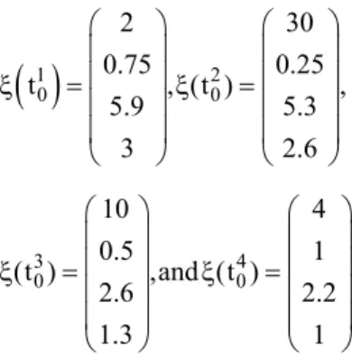
In order to generate data for parameter identification, four experiments are simulated with a

constant dilution rate ( D=0.1) and a constant input concentration (S_in=10), starting from the following known initial conditions:

( )

1 2

0 0

3 4

0 0

2 30

0.75 0.25

t , (t ) ,

5.9 5.3

3 2.6

10 4

0.5 1

(t ) , and (t ) .

2.6 2.2

1.3 1

⎛ ⎞ ⎛ ⎞

⎜ ⎟ ⎜ ⎟

⎜ ⎟ ⎜ ⎟

ξ = ξ =

⎜ ⎟ ⎜ ⎟

⎜ ⎟ ⎜ ⎟

⎝ ⎠ ⎝ ⎠

⎛ ⎞ ⎛ ⎞

⎜ ⎟ ⎜ ⎟

⎜ ⎟ ⎜ ⎟

ξ = ξ =

⎜ ⎟ ⎜ ⎟

⎜ ⎟ ⎜ ⎟

⎝ ⎠ ⎝ ⎠

(28)

Each experiment lasts 20 days and the whole state vector is measured daily. Measurements are affected by a zero-mean, Gaussian noise, characterized by a relative standard deviation of σ =_r 10%. The experimental datasets are systematically interpolated by cubic smoothing splines via the csaps function of Matlab, choosing p=0.15 as the smoothing parameter (Fig. 1).

The experimental data and their interpolation are then treated by the two-step stage of our identification procedure without any extra filtering. In order to make performance comparisons, these data are also treated with a classical optimization algorithm that attempts to identify all the unknown parameters in a single step.

Brazilian Journal of Chemical Engineering Vol. 27, No. 03, pp. 381 - 390, July - September, 2010 Benchmark Statement and Results

Initial guesses of the parameters are randomly generated at increasing distances from their optimum value ϑ* through the following formula:

(

)

*

0 1 Δ ,

ϑ = ϑ + ϑα (29)

where α is a standard normally distributed random vector and Δϑ is an initial level of uncertainty that successively takes 1000 increasing values that are equally-spaced over the range [0,1.5[ . Numerical problems are prevented by simply forcing the positivity of the initial guesses of the kinetic parameters.

Since no prior information is available on the stoichiometry of the system, the stoichiometric matrix K is estimated through (20). All the _a optimizations are performed with the Nelder-Mead simplex algorithm implemented in the Matlab function fminsearch. This optimizer indeed offers the advantage of being more robust than classical gradient-based algorithms with regard to the presence of local minima in the cost function.

In order to illustrate the performances of our identification procedure, the distance that separates the estimates from the true parameter value has been computed and is represented as histograms in Fig. 2. For both approaches, i.e., the direct identification of

all the parameters and the two-step procedure, the following relative Euclidian distance is chosen:

( )

*

* i i

* i i

d ϑ ϑ =, ⎛_⎜⎜ϑ − ϑ ⎞_⎟⎟. ϑ

⎝ ⎠

∑

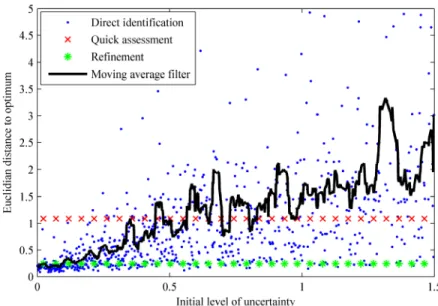
(30)

While the estimates resulting from the direct identification approach are widely distributed over the range of relative distances, the quick assessment step visibly has a gathering effect on their distribution. This highlights the presence of a strongly-attractive, global minimum in the cost function (21), which leads to convergence even from poor initial guesses. The second step of our procedure then clearly refines the result by removing the remaining bias from the solution vector. Fig. 3 confirms this explanation by showing the influence of the initial uncertainty level on the optimality of the estimates for both approaches.

Since it operates on a restricted set of parameters and requires no numerical integration of the model differential equations, the quick assessment step usually converges within a fraction of a second. This is extremely fast in comparison with the seconds or minutes required for other classical optimization methods to converge. A plot of the computation time as a function of the initial uncertainty level illustrates these observations for both identification approaches (Fig. 4).

Figure 3: Evolution of the distance separating the estimates from their optimum value as a function of the initial uncertainty level Δϑ of the parameters, for both identification approaches. A moving average filter with a 20-sample time window shows the increasing tendency for the direct approach.

Figure 4: Evolution of the computation time as a function of the initial uncertainty level Δϑ of the parameters, for both identification approaches. A moving average filter with a 20-sample time window shows the increasing tendency for the direct approach.

CONCLUSIONS

The systematic identification procedure presented in this paper uses and extends previous research results to the transformation of C-identifiable reaction schemes into biologically-consistent

Brazilian Journal of Chemical Engineering Vol. 27, No. 03, pp. 381 - 390, July - September, 2010 continuous culture of microalgae highlights the

robustness of the new procedure with regard to uncertainties in the initial guess.

Further research is still required, though, to characterize better the influence of biological constraints on the convergence of the identification algorithm. In particular, the choice of an appropriate structure for the expression of the reaction rates is a challenging issue that could still improve the applicability of our methodology.

ACKNOWLEDGEMENTS

Johan Mailier is a Research Fellow of the National Fund of Scientific Research (FNRS – Belgium). This paper presents research results of the Belgian Network DYSCO (Dynamical Systems, Control, and Optimization), funded by the Interuniversity Attraction Poles Programme, initiated by the Belgian State, Science Policy Office. The scientific responsibility rests with its authors.

NOMENCLATURE

,

A B Dynamic models of bioprocesses B, B Metabolized substrate (concentration) C Pseudo-stoichiometric submatrix that is

part of a C-identifiable scheme l

C Estimation of matrix C

*

d( ,ϑ ϑ ) Relative Euclidian distance between parameter vectors ϑ and ϑ*

D Input dilution rate

F Vector of external feed rates

a b

F , F Subvectors of external feed rates

M

I Identity matrix of size M

J Cost function

K Pseudo-stoichiometric matrix

a b

K , K Pseudo-stoichiometric submatrices la

K Estimation of the pseudo-stoichiometric submatrices

K_A Pseudo-stoichiometric matrix of model A K_B Pseudo-stoichiometric matrix of model B M Number of macroscopic reactions

*

M Optimum number of macroscopic reactions N Number of key-components

e

N Number of experiments

e s

N Number of samples taken during the eth experiment

p _{Smoothing parameter for Matlab function}

csaps

P Matrix of eigenvectors

k

P Set of the products of the kth reaction Q Regular transformation matrix R, R Intracellular substrate (concentration)

k

R Set of the reactants of the kth reaction S,S Extracellular substrate (concentration)

in

S Substrate feed concentration

e k

t kth time instant of the eth experiment

e 0

t Initial time of the eth experiment

u(t) Measured vector interpolated and filtered at time t

U Matrix of measured vectors

w(t) Non-measured vector interpolated and filtered at time t

W Matrix of non-measured vectors X, X Biomass (concentration) z Transformed state vector

α Standard normally distributed random vector

Δϑ Initial level of uncertainty of the parameter vector

ϑ Parameter vector

*

ϑ Optimum parameter vector

i

ϑ ith element of vector ϑ

* K

ϑ Vector of the optimum stoichiometric parameters

a

K

ϑ Vector of the parameters related to K _a

a

* K

ϑ Vector of the optimum parameters related to K a

a

* K ,i

ϑ ith element of a

* K

ϑ

0

ϑ Initial guess of the parameter vector ϕ

ϑ Vector of the kinetic parameters _ϕ

ϑ Estimation of the vector of the kinetic parameters

*

ϕ

ϑ Vector of the optimum kinetic parameters

* ,i

ϕ

ϑ ith element of ϑ*_ϕ

*k

ν Pseudo-stoichiometric coefficient of the kth reaction

ξ State vector composed of the reacting species concentrations

a, b

ξ ξ State subvectors of the reacting species concentrations

i

ξ ith element of the state vector

r

σ Relative standard deviation

ϕ_A Reaction rate vector of model A ϕ_B Reaction rate vector of model B

C

ϕ Reaction rate vector of a C-identifiable scheme

k

ϕ kth element of the reaction rate vector

REFERENCES

Bastin, G. and Dochain, D., On-line Estimation and Adaptive Control of Bioreactors. Elsevier Science Ltd, New York (1990).

Bernard, O. and Bastin, G., On the estimation of the pseudo-stoichiometric matrix for macroscopic mass balance modelling of biotechnological processes. Mathematical Biosciences, 193, No. 1, 51 (2005a).

Bernard, O. and Bastin, G., Identification of reaction networks for bioprocesses: determination of an incompletely known pseudo-stoichiometric matrix. Bioprocess and Biosystems Engineering, 27, No. 5, 293 (2005b).

Bogaerts, Ph., Delcoux, J.-L. and Hanus, R., Maximum likelihood estimation of pseudo-stoichiometry in macroscopic biological reaction schemes, Chemical

Engineering Science, 58, No. 8, 1545 (2003). Bogaerts, Ph., Rooman, M., Vastemans, V. and Vande

Wouwer, A., Determination of macroscopic reaction schemes: towards a unifying view. Proceedings of the 17th World Congress of IFAC. Seoul (2008).

Chen, L. and Bastin, G., Structural identifiability of the yield coefficients in bioprocess models when the reaction rates are unknown. Mathematical Biosciences, 132, No. 8, 35 (1996).

Delcoux, J.-L., Hanus, R. and Bogaerts, Ph., Equivalence of reaction schemes in bioprocesses modelling. Proceedings of the 4th International Symposium on Mathematical Modelling and Simulation in Agricultural and Bio-Industries. Haifa (2001).

Hulhoven, X., Vande Wouwer, A. and Bogaerts, Ph., On a systematic procedure for the predetermination of macroscopic reaction schemes. Bioprocess and Biosystems Engineering, 27, No. 5, 283 (2005). Lemesle, V. and Mailleret, L., A mechanistic

investigation of the algae growth "Droop" model. Acta Biotheoretica, 56, No. 1-2, 57 (2008).