Investigation and Characterization of materials towards building ionization vacuum gauges

Ivo Guilherme Correia Figueiredo

Licenciado em Engenharia Física

Investigation and Characterization of

materials towards building ionization

vacuum gauges

Dissertação para obtenção do Grau de Mestre em

Engenharia Física

Orientadores: Prof. Doutor Orlando Teodoro

Doutor Nenad Bundaleski

Júri:

Presidente: Prof. Doutora Isabel Catarino

Arguente: Prof. Doutora Susana Sério Vogal: Doutor Nenad Bundaleski

Investigation and Characterization of materials towards building ionization vacuum gauges

Copyright © Ivo Guilherme Correia Figueiredo, Faculdade de Ciências e Tecnologia, Universidade Nova de Lisboa.

Acknowledgements

Foremost I would like to thank Dr. Nenad Bundaleski for the immense help he provided me during the course of my thesis. His guidance and insight proved critical towards reaching the goals initially proposed, and his optimistic outlook helped me endure through the several setbacks that occurred throughout these six months. I would also like to thank Prof. Orlando Teodoro for approaching me to work on this thesis providing me the opportunity to work on his lab. His knowledge in this field proved enlightening and allowed me to learn the workings of a physics lab.

I would like to extend my gratefulness to Afonso Moutinho, for his massive contribution to solving the electronics issues which were common during my work, as well as Ana Fonseca for her help both in the lab and in writing this thesis. Furthermore, I would like to thank my friends Ricardo Silva and Francisco Canhoto for putting up with me for five long years and for incentivizing me to display some much-needed effort in studying, as well as my colleagues that worked on the CEFITEC Surface Science lab with me, namely Cristiano Dionisio, Rubén Aguincha and Gonçalo Alves, all of which allowed for a pleasant work environment.

i

Resumo

O manómetro de ionização é um dos medidores de pressão mais utilizados para medição de pressões baixas. Em teoria este tipo de dispositivos poderia ser utilizado para medir pressões extremamente baixas. No entanto, quando utilizados para medir pressões mais baixas estes manómetros sofrem de problemas de estabilidade levando a um acréscimo da incerteza da medição, que por sua vez limita a gama de pressões de trabalho. Apesar dos processos que influenciam a estabilidade destes sistemas serem bem conhecidos, pouco estudo foi feito com vista a melhorar o próprio sistema. De encontro com o projeto europeu EMPIR “Towards a documentary standard for an ionization vacuum

gauge”, este trabalho tem como objetivo propor materiais mais adequados para utilização em todo o tipo de manómetros de ionização. Dito isto, este projeto foca-se no estudo de um dos maiores problemas que afetam a estabilidade das medições feitas com manómetros de ionização, nomeadamente a produção de eletrões secundários induzida por iões (IISEY), através da medição da função de trabalho e da degradação da superfície antes e após a exposição a condições idênticas às observadas em manómetros de ionização de diferentes materiais e correlacionar estes parâmetros com as medições de IISEY.

Dos materiais candidatos foram escolhidos o molibdénio, ouro e aço inox. Em todos os casos tornou-se evidente que contaminação do elétrodo coletor por carbono é inevitável, mesmo em condições limpas. Esta contaminação tem origem no interior do próprio material, no caso de materiais técnicos, e maioritariamente na grelha atrativa. Em geral, aumento de carbono resulta numa redução de IISEY. Chegou-se à conclusão que a IISEY é altamente influenciada pelas condições superficiais. Como tal, trabalhar com espécies exóticas levará a eventual adesão de diferentes compostos, levando a alterações de IISEY. Embora não conclusivo, o inox e o ouro aparentam ser os mais indicados dentre os candidatos.

iii

Abstract

Ionization gauge systems are one of the most frequent types of pressure measurement devices used for measuring very low pressures. In theory this type of devices could be used to measure extremely low pressures. However, when working in the lower end of the pressure range the ionization gauges suffer from stability issues leading to an increase in measurement uncertainty, which in turn limits the pressure work range. While the processes that influence the stability of these systems are fairly well known, not much has been done towards improving the actual systems. In line with the European EMPIR project “Towards a documentary standard for an ionization vacuum gauge”, this project aims towards proposing materials better suited for usage in regular ionization gauges. With that said, the project will focus on the study of one of the most pressing problems regarding the stability of the measurements made with ionization gauges, namely Ion Induced Secondary Electron Yield (IISEY) from ion collectors, by

measuring the sample’s work function and surface degradation before and after exposure to environments similar to those present in ionization gauges and correlate them to measurements of the IISEY obtained mid exposure.

Different candidate materials were chosen, namely molybdenum, gold and stainless steel. In all cases it became evident that carbon contamination is an inevitable occurrence in the collector electrode, even in clean environments. This contamination was deemed to originate from the material itself, in technical materials, and mainly from the filament and the grid electrode. In general, carbon content increase meant a decrease of IISEY. IISEY was deemed heavily influenced by surface conditions. As such, working with exotic species should provide adhesion of different compounds, therefore changing the IISEY. While not conclusive, stainless steel and gold seem to be the better suited of the candidate materials.

v

Index

Figure List ... vii

Table list ... ix

List of Symbols and Abbreviations ... xi

1.

Introduction ... 1

2.

Fundamental Concepts ... 5

2.1.

Ion Induced Secondary Electron (IISEY) ... 5

2.2.

X-Ray Spectroscopy (XPS) ... 8

2.3.

Residual Gas analysis ... 11

2.4.

Work Function (WF) measurement ... 11

2.5.

IISEY measurement ... 13

3.

State of the art

–

Instabilities of the ionization gauges related to IISEY from a collector .. 15

4.

Experimental Setup ... 17

4.1.

Experimental Equipment ... 17

4.2.

Repairs and improvements of the existing setup ... 19

4.2.1.

Reconstruction of the fast entry lock pumping system ... 20

4.2.2.

Reconstruction of the detection electronics ... 21

4.2.3.

Design of the new acquisition system for the RGA ... 22

4.3.

Experimental Procedures ... 23

5.

Results ... 27

5.1.

Mass Analysis of the gas in the IGS ... 27

5.2.

Influence of the material exposure to the IGS discharge on the surface composition

30

5.2.1.

Molybdenum ... 30

5.2.2.

Gold ... 34

5.2.3.

Stainless Steel ... 34

5.3.

Influence of the Ar discharge exposure on the sample work function ... 38

5.4.

IISEY before and after the exposure ... 40

5.5.

Contamination analysis ... 44

5.6.

Long exposure ... 46

6

Conclusions ... 49

vii

Figure List

Figure 1.1: Scheme of an Bayard-Alpert (BA) gauge, a type of Ionization gauge [2]. ... 1

Figure 1.2: X-Ray Photoelectric Effect in Ionization gauges. ... 2

Figure 1.3: Electron Stimulated Desorption of neutral (1) and ionic (2) species. ... 2

Figure 2.1: Energy diagram illustrating Auger Neutralization process [6]. ... 6

Figure 2.2: Comparison of IISEY of clean and contaminated metals [13]. ... 7

Figure 2.3: X-Ray Photoelectron Spectroscopy setup [24]. ... 10

Figure 2.4: QMS schematics [26]. ... 11

Figure 2.5: Measurement of energy cutoff of the gold sample. ... 12

Figure 2.6: Work function measurement setup. ... 13

Figure 4.1: XSAM system used for this project. ... 17

Figure 4.2: Schematic of the Ionization Gauge Simulator. ... 18

Figure 4.3: Introduction and Preparation chambers vacuum setup. Modifications are highlighted in red. ... 20

Figure 4.4: RGA control software interface. ... 23

Figure 4.5: IISEY measurement setup. ... 25

Figure 4.6: IGS electric connections and sample positioning. ... 25

Figure 5.1: Mass spectrum of the gas after Argon introduction into the IGS. ... 27

Figure 5.2: Mass spectrum of the gas after residual gas introduction in IGS. ... 28

Figure 5.3: Mass spectrum of the residual gas with IGS Off and On. ... 29

Figure 5.4: Mo 3d5/3 line before the exposure to the Ar discharge. ... 31

Figure 5.5: Mo 3d5/3 line after the exposure to the Ar discharge. ... 32

Figure 5.6: C 1s line before the exposure to the Ar discharge. ... 33

Figure 5.7: C 1s line after the exposure to the Ar discharge. ... 33

Figure 5.8: Au main peak. ... 34

Figure 5.9: SS’s O 1s line before exposure. ... 35

Figure 5.10: SS’s O 1s line after exposure. ... 35

Figure 5.11: SS’s Cr 2p3/2 line before exposure. ... 36

Figure 5.12: SS’s Cr 2p3/2 line after exposure. ... 37

Figure 5.13: Mo secondary electron spectrum. ... 38

Figure 5.14: Au secondary electron spectrum. ... 39

Figure 5.15: SS secondary electron spectrum. ... 39

Figure 5.16: Molybdenum IISEY before and after exposure. ... 41

Figure 5.17: Gold IISEY before and after exposure. ... 41

Figure 5.18: Stainless steel IISEY before and after exposure. ... 42

Figure 5.19: Evolution of the IISEY of gold with repeated exposure... 43

Figure 5.20: Cu survey after prolonged exposure. ... 46

ix

Table list

Table 5.1: Elemental quantification of the XPS spectrum for each sample. ... 38

Table 5.2: Energy cutoff before and after exposure. ... 40

Table 5.3: Gold surface composition with exposure. ... 43

Table 5.4: Relative intensity of each carbon contribution. ... 44

Table 5.5: Copper surface composition throughout cleaning. ... 44

Table 5.6: Surface composition after different sample exposures. ... 45

xi

List of Symbols and Abbreviations

𝐸

𝑡ℎ – Kinetic emission energy threshold

𝐸

_𝑘 – Kinetic energy

𝑀

𝑖 – Ion Mass

ℎ𝜈

– Photon energy

𝑚

𝑒 – Electron Mass

𝐸

_𝑏 – Binding energy

𝐸

_𝑓 – Fermi Energy

𝐴

_𝑋 – Relative concentration of element X

𝑊

𝑓 – Work Function

𝐼

_𝑋 – X element peak area

ɣ

– IISEY

𝑅𝑆𝐹(𝑋)

– Relative sensitivity factor of element X

𝐸

_𝑖

– Ionization Energy

𝐸

_𝑐

– Secondary electron energy cutoff

IG

– Ionization Gauge

HV

– High Vacuum

UHV

– Ultra High Vacuum

XHV

– Extreme High Vacuum

BA

– Bayard-Alpert

XP

– X-ray Photoelectric effect

ESD

– Electron Stimulated Desorption

IISEY

– Ion induced secondary electron yield

XPS

– X-Ray Photoelectron Spectroscopy

WF

– Work Function

RGA

– Residual Gas Analyzer

QMA

– Quadrupole Mass Analyzer

SS

– Stainless Steel

IGS

– Ionization Gauge Simulator

1

1. Introduction

During the last decades the technology surrounding vacuum production has been steadily improving, reaching pressures as low as 10-14 _{mbar [1]. However vacuum measurement}

devices haven’t accompanied the evolution of vacuum production systems.

One of the most used devices for measuring hard vacuums are the Ionization Gauges (IG) given their versatility and large range of pressure measurements, covering High Vacuum (HV), via Ultra High Vacuum (UHV), to Extreme High Vacuum (XHV). Ionization gauges are characterized in accord to how the ionization occurs, whether with an electron emitting filament (hot cathode ionization gauges) or without it (cold cathode ionization gauges). This study will focus on the first type.

Figure 1.1: Scheme of an Bayard-Alpert (BA) gauge, a type of Ionization gauge [2].

Although several configurations of hot cathode ionization gauges exist, all of them share the same working principle (Figure 1.1). Electrons produced in the filament are attracted to a grid gaining energy. These electrons then collide with the residual gas particles, ionizing them. The ions are then attracted to the collector electrode. The measured ion current is proportional to the amount of the gas in the chamber, therefore allowing for pressure measurements.

2 Photoelectric (XP) effect in the collector, Electron Stimulated Desorption (ESD) from the grid and Ion Induced Secondary Electron Yield (IISEY) from the collector are the most important [3].

XP, illustrated in Figure 1.2, occurs as a result of high energy electrons colliding with the grid. When this happens, X-rays are produced, which can then irradiate a material and produce secondary electrons by a photo effect. When this happens on the collector, an additional current will be measured of the same sign as the ion current, providing virtually higher pressure reading than the actual one. Since X-ray creation will mostly predominantly happen in the vicinity of the grid, several IG designs manage to limit XP contribution by hiding the collector from the grid [3].

Figure 1.2: X-Ray Photoelectric Effect in Ionization gauges.

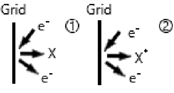
As the name implies, ESD is a result of interaction between an electron and a surface. By coming into close proximity with a surface, the electron projectile can excite the surface atoms. The energy gained by said atoms is related to the minimum distance between it and the incoming electron. If enough energy is gained during this interaction, the atom can then be expelled from the surface as a neutral or ionic species (Figure 1.3). These species will eventually end up in the collector due to its charge, providing measurement uncertainty not unlike XP [3].

3 IISEY is a process which occurs on ion-surface collisions. In it, the incoming ion is neutralized, resulting in the emission of an electron from the surface. This is a result of a combination of different phenomena with potential and kinetic energy origin, all of which will be described in more detail in the next chapter.

XP and ESD are not pressure dependent, which results in a fixed error of the readings throughout overall pressure range. This means that these mechanisms produce consistently higher pressure that the actual one in the chamber, which only becomes a concern when working at sufficiently low pressures. IISEY however is proportional to the pressure in the chamber, meaning that it produces the same relative error in both HV and XHV range. This results in added measurements’ uncertainty. While the effects of the photoelectric effect can be mostly solved by hiding the collector from the grid, IISEY and ESD are more closely related to the materials. Therefore, by properly studying the changes of IISEY and ESD in different kinds of materials we can get better insight into which materials are better suited for usage in ionization gauges and, as a result, further extend the working range and the stability of these devices.

Unlike ESD, the existence of IISEY does not impose a direct measurement issue, since this effect can be taken into account via proper calibration. However, if IISEY of different ions is changing while the ionization gauge is operating, this presents a major problem since the conversion from current to pressure (i.e. ionization gauge sensitivity) is changing as well. With this in mind, the major idea of the project is to measure the changes in IISEY of different samples exposed to conditions similar to those in IG. The considered materials will be the candidates for the collector of ionization gauges, such as Au, Mo, etc. Due to the low ion energies reached in ionization gauges (i.e. 100 to 300 eV), IISEY is a process which will only take place at the first atomic layer, and mainly caused by the so-called potential electron emission. As such, it is strongly affected by the work function of the sample [4], the latter being dependent on the surface conditions, such as adsorption of different impurities. Consequently, Work function change of the samples will be measured before and after the exposure, with the goal of correlating work function changes with IISEY variations in to IG environment. Additionally, the samples surface will be analyzed with X-Rays Photoelectron Spectroscopy (XPS), to gain further insight into the surface modifications induced by the exposure.

5

2. Fundamental Concepts

2.1. Ion Induced Secondary Electron (IISEY)

At first glance the process of IISEY appears to be purely related to the momentum transfer between ions and electrons and as such a strictly kinematic phenomenon. This type of process, in which kinetic energy of projectiles are used to excite electrons, is known as kinetic electron emission. Taking into consideration the approximations of the band theory, which states that the valence electrons of a metal can be considered as free electrons with varying levels of kinetic energy, ranging from zero to the Fermi energy (Ef) in respect to the bottom of

valence band, minimum ion projectile kinetic energy for which IISEY could occur can be calculated as

𝐸

_𝑡ℎ

≈

𝑀𝑖

2𝑚𝑒

[𝐸

𝑓

− √𝐸

𝑓

(𝐸

𝑓

+ 𝑊

𝑓

) +

𝑊𝑓

2

]

(2.1)

,with 𝐸_𝑡ℎ being the energy threshold, 𝑊_𝑓 the metal work function, 𝑀_𝑖 the ion mass and 𝑚_𝑒 the

electron mass. In the case of Al (Ef = 10.6 eV, Wf= 4.3 eV) this threshold energy can be

calculated to be 170 eV/u [5], whilst for gold it would be 270 eV/u when taking into consideration the effective mass of the electrons in gold [6]. Taking this information into account and considering the energy ranges in typical ionization gauge (up to 300 eV), it can be expected that most of the IISEY kinetical contributions are a result of hydrogen ion collisions, which coincidentally makes up most of the residual gas in the ultra-high vacuum range.

If only this kinetic mechanism is taken into consideration, it would be expected that IISEY for a particular ion would only occur above the energy threshold. However empirical data showed that IISEY also occur for most of the ions at energies below the threshold at a nearly constant rate. To fully explain the process of IISEY a potential energy of projectiles should be also considered. Process at which electrons are excited and eventually emitted using the projectile potential energy is known as potential electron emission.

One of the key aspects of this type of interactions is that the rate of potential electron emission is independent of the kinetic energy of ions. The first relevant model of this process was introduced by Hagstrum in 1954 [7]–[9]. This model stipulates that an ion can be neutralized through two distinct non-radiative processes in an ion-metal collision scenario.

6 responsible for most of the potential IISEY for atoms with high ionization potential Ei, such as

noble gases.Typical example of such neutralization process is interaction of slow He+ _{ions with} metals. Assuming that the ion energy levels remain unchanged throughout the collision, the condition for electron emission through this process is Ei>2Wf.

Figure 2.1: Energy diagram illustrating Auger Neutralization process [6].

On the other hand, if the projectile has unoccupied energy levels comprised in between the bottom of the valence band and the Fermi level of the metal, another process can occur. In this case, Resonant Neutralization (RN) takes place, in which a valence electron of the metal occupies this excited state of the projectile. Due to the natural tendency of matter to achieve better stability, the excited neutral projectile quickly decays in an Auger deexcitation process (AD): the energy gained by the deexcitation of the neutral is spent on the emission of an electron from the valence band or from the projectile single electron state above the valence level. This scenario is characteristic in Ne+ _{collision with metals.}

Both processes take place with transition rates of the order of 10-15 _{s. Since these rates} are similar to the duration of a single binary collision in this energy range, these phenomena can be expected to occur with high probability during the interaction of projectile with the first atomic layer. This was experimentally proved by Hagstrum [10].

Based on the simple assumptions introduced by Hagstrum in his original model (such as application of bulk parameters and assumption of uniform density of states [8]) Kishinevsky formulated the following relation between the ion induced secondary electron yield γ [11]:

7 Using known experimental data, Kishinevsky estimated the values of the parameters α and β to be 0.2/Ef and 0.8. Taking the same approach and by using a different set of

experimental data, Baragiola and co-workers obtained very good agreement for α = 0.032 eV-1 and β = 0.78 [12].

While taking all the above processes allowed for a better approximation the empirical data, it became evident that there were still unknown factors in play since the experimental data exhibited an energy dependence of the IISEY well below the expected kinetic energy threshold. In particular, this process is observed mainly in unclean or otherwise contaminated metallic surface.

Figure 2.2: Comparison of IISEY of clean and contaminated metals [13].

Further investigation revealed that ion induced secondary electron emission was also being observed when atomic projectiles were used, despite them having zero potential energy, which led researchers to believe that another, yet unknown mechanism driven by the projectile kinetic energy was happening at subthreshold energies. This was later explained as being originated from transiently formed autoionizing quasimolecules [6], [14]. This effect was first observed and explained by Fano and Lichten while studying Ar-Ar collisions in gas phase, culminating in the development of the electron promotion model for this type of collisions [15]. This model was expanded in order to include asymmetric collision in the work done by Barat and Lichten [16].

8 or more electrons by Auger Effect. While this phenomenon was explained for atom-atom collisions in gas phase, the same result can be obtained in atomic projectile collisions with atoms of a solid.

The energy threshold for this process is related to the minimum distance between the interacting atoms. This model was clearly confirmed in a detailed study of Li and Ar ions colliding with clean Al metal, secondary electron emission originates from Al atoms previously highly excited in binary collisions with the projectiles [17].

2.2. X-Ray Spectroscopy (XPS)

X-Ray Spectroscopy is a technique that allows quantitative analysis of the surface composition of all sorts of materials. This method takes advantage of the well know Photoelectric Effect in which electrons are emitted due to the absorption of light of a certain wavelength by a material [18]. The energy of these electrons is determined by the type of radiation and material in question, being expressed by the following formula

𝐸

_𝑘

= ℎ𝜈 − 𝐸

_𝑏

− 𝑊

_𝑓𝑠𝑎𝑚𝑝𝑙𝑒 (2.3)

where 𝑬_𝒌 is the kinetic energy of electrons inside the analyzer, 𝒉𝝂 is the photon energy, 𝑬_𝒃 is the binding

energy of the level from which the electron was excited measured in respect to the Fermi level, and

𝑾_𝒇𝒔𝒂𝒎𝒑𝒍𝒆 is the work function of the analyzer. By measuring the electron kinetic energy while knowing the

incident radiation one can determine its binding energy. Since the binding energy is a characteristic property of an atom, this can be used to characterize the irradiated material. XPS works by constantly bombarding the sample with a known wavelength radiation while scanning the emitted electrons by energy, therefore producing an energy spectrum.

Given the nature of this phenomenon, electrons that are emitted from the inner layers of a material are more likely to lose part of their energy by interacting with the valence electrons of the sample. These electrons, if detected, no longer have information regarding the surface composition [19]. They instead contribute to the spectrum background. Because of this, XPS is mainly used to analyze the surface of a material, although different setups can be used to scan deeper layers.

9 binding energies. The chemical peak shift is used for the bond identification. In addition, mere shape of the photoelectron lines can be sometimes used as a fingerprint of the chemical environment [20], due to the presence of shake-up satellites or other effects such as multiplet splitting. Such specific shapes are usually fitted by the superposition of different peaks having well-defined constraints (i.e. relative positions intensities and widths) [21], [22].

Alongside the photoelectron peaks, other lines can be observed which are a result of the Auger emission. When an electron from lower energy levels is removed from an atom due to the Photoelectric Effect, an electron from the higher bands will decay to take its place. The excess energy can be released by radiation or emission of an Auger electron. In the latter case, which is usually much more probable, this

electron carries information of the atom’s energy levels, and can be therefore used for the elemental identification.

Rough quantification of surface elemental composition can be achieved using the following equation

𝐴

_𝑋

=

𝐼𝑋 𝑅𝑆𝐹(𝑋)

∑𝑛_{𝑖𝑅𝑆𝐹(𝑖)}𝐼𝑖 (2.4)

in which 𝐴_𝑋, 𝐼_𝑋 and 𝑅𝑆𝐹(𝑋) being the relative concentration, the peak area after removal of the background and the Relative Sensitivity Factor of an element X, respectively. It should be stressed that XPS quantification using eq. (2.4) can be performed only in the case of a single-phase systems. In other cases, more complex approaches are necessary.

10 Figure 2.3: X-Ray Photoelectron Spectroscopy setup [24].

XPS equipment, presented in Figure 2.3, is a three-part system comprised of the X-Ray source, an energy analyzer and the detector. The X-Ray sources rely on the fact that when high energy electrons collide with a solid (anode in our case) characteristic radiation is emitted. Alongside with an energy continuum, the majority of the radiation is within a small wavelength range, providing almost fixed energy radiation source. Further improvements can be achieved through the usage of X-ray monochromators. Anodes are typically made of magnesium or aluminum [25]. Energy analyzers use electric field in order to scan the incoming electrons. The most common setup is the hemispherical energy analyzer. Electrons entering this device have their trajectories bent due to the electric field present between the hemispherical electrodes. The electrode voltages are adjusted so that only electrons with a selected energy can reach the detector. The energy resolution of these devices is proportional to the voltages used. Different parts of a spectrum will have different resolutions. To avoid this, most XPS systems work in Fixed Analyzer Transmission (FAT) mode which uses an array of lenses to decelerate the electrons, while maintaining the analyzer’s pass energy constant. Typical detectors are channeltrons or channelplates. Both of these rely on channels made up of materials with high secondary electron yields. When an electron coming from the analyzer collides with the

channel’s walls a chain reaction occurs where electrons are successively multiplied. These make up a measurable current which is then transformed into digital data in the preamplifiers.

11

2.3. Residual Gas analysis

Mass spectroscopy is a technique which allows elemental and molecular identification by taking advantage of their mass difference. In this study, mass spectroscopy was performed using a Residual Gas Analyzer (RGA), more precisely the QMG421 mass analyzer produced by Balzers. This device works by ionizing the gas in a chamber and then measuring the resulting ions mass using a Quadrupole Mass Analyzer (QMA). The ionization is performed through the usage of an electron emitting filament and an anode which produce electrons with energies up to 140 eV. The electrons are colliding with the gas inside the ionizing chamber and create ions, which are then accelerated towards the mass analyzer (Figure 2.4). This setup is remarkably similar to the one used in IGs and as such should provide insight into the ions produced in an IG environment. Mass measurement is performed using a quadrupole. This device is comprised of four parallel long electrodes and a detector, in this case a Faraday cage. Pairs of opposing electrodes are in a shortcut. The voltage applied between them is a combination of AC and DC components. Ions having the same energy, but different masses enter the quadrupole mass analyzer. For a set of AC/DC voltages only ions with a certain mass to charge ratio will be able to traverse the quadrupole path, therefore reaching the detector. A QMA works by scanning the voltages (either by changing the frequency or the voltage module) and measuring the current reaching the detector. The results are often represented in a form of counts vs mass/charge ratio.

Figure 2.4: QMS schematics [26].

2.4. Work Function (WF) measurement

12

𝐸

_𝐶

= 𝑊

_𝑓𝑠𝑎𝑚𝑝𝑙𝑒

− 𝑊

_𝑓𝑎𝑛𝑎𝑙𝑦𝑧𝑒𝑟 (2.5)

where is 𝑊_𝑓𝑠𝑎𝑚𝑝𝑙𝑒 the sample work function and 𝑊_𝑓𝑎𝑛𝑎𝑙𝑦𝑧𝑒𝑟 is the analyzers work function. Since

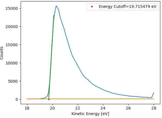
the work function of the analyzer is a static value (it is not supposed to be changing during the ongoing experiments), changes in the sample work function will be observed as shifts of the energy cutoff. Therefore, following the energy cutoff shift of any secondary electron emission spectrum gives us direct insight into the changes of the sample work function.

However, one should have in mind that only electrons with 𝐸_𝐶 > 0 eV will be able to

reach the detector. If 𝑊_𝑓𝑠𝑎𝑚𝑝𝑙𝑒 < 𝑊_𝑓𝑎𝑛𝑎𝑙𝑦𝑧𝑒𝑟, the cutoff will always be at Ec = 0 eV, and the

changes of the sample work function will not be observable. This is why the sample is always negatively biased in these measurements ( -20.0 V in our case) to ensure repulsion of all electrons from the sample.

The setup used for the sample work function change measurement is schematically presented in Figure 2.6. In our realization of the sample work function change measurements, the X-ray source was used to induce secondary electron emission through the photoelectric effect from the biased sample. Secondary electron spectra were measured before and after different sample treatments in order to measure the energy cutoff, and consequently determine the work function changes.

13 Figure 2.6: Work function measurement setup.

2.5. IISEY measurement

The measurement of IISEY was accomplished through biasing the sample while under ion bombardment. When the sample was positively biased, the current measurement represents only the ion current reaching the sample since secondary electrons that would normally leave the surface will encounter a potential barrier and therefore remain in the sample. On the other hand, if the sample is negatively biased both the ion current and the leaving electron current will be measured. Furthermore, this biasing allows for repulsion of additional generations of electrons resulting from the ion bombardment. The ratio between these two measurements constitutes the IISEY value.

IISEY measurements proved difficult to obtain due to the space charging effects. Higher currents are more reliably measured. However, increasing the number of generated ions lead to the problems in ion extraction due to the space charging. Furthermore, this space charge means that the ions will have slightly bent trajectories which could mean that they miss the

E

A

_{= E}

kS

+ WF

sample

–

WF

analyzer

+ 20V

E

A

_{= E}

14 sample. Taking this into account, IISEY measurements were done with ion currents in the nA range, using a high precision electrometer.

15

3. State of the art

–

Instabilities of the ionization gauges related to

IISEY from a collector

Although the phenomenon of potential electron emission is generally understood since fifties, i.e. at the same time when Bayard-Alpert type of Ionization gauges was invented, the influence of IISEY from the collector on the IG instabilities was typically considered to have secondary significance. Indeed, there are only few studies of this phenomenon in IGs, typically performed during eighties or even earlier. However, in the “EMPIR Towards a documentary

standard for an ionization vacuum gauge” project this issue is found to be particularly important, along with other well-known effects (such as electron trajectory and length distribution), in order to achieve the basic aim: finding a new generation of IGs providing 1 % long term stability.

It is known that long term operation of ionization gauges improves their stability and reduces the sensitivity of the system. The viability of tungsten and platinum for usage as the collector material, regarding its work function was studied in [27]. Using Auger Electron Spectroscopy, it was found out that the main contaminants present in the materials when exposed to air were O and C, for tungsten, and C, O, S, K, Ca and Ag, for platinum. After proper cleaning by annealing, they recorded an increase in the work function of 0.7 eV and 0.6 eV of tungsten and platinum, respectively. According to the Hagstrum theory, work function increase leads to a reduction of IISEY (eq. 2), which explains reduction of the detector sensitivity along the operation.

Another research led by Gentsch and co-workers proposed another configuration of IG, namely Screened Ionization Gauge (SIG), with all the electrodes being coated with gold [28]. This setup provided well defined ionisation path lengths (another important source of beam instabilities) and clean electrode surface (whilst operating at 250 °C), which guaranteed a stable work function and therefore stable IISEY. The study reported that when using a platinum collector, IISEY was changing during the operation due to the alloying of gold by the supported material. With this in mind, tungsten was concluded to be a better suited material since gold

isn’t soluble in tungsten.

17

4. Experimental Setup

This chapter is dedicated to the overview of the experimental setup, as well as the experimental procedures adopted throughout this study. In addition, repairs and improvements of the systems are also listed and described in this chapter.

4.1. Experimental Equipment

In order to obtain reliable results this study had to be done in a clean environment. Therefore, a three-part UHV system XSAM 800 (Figure 4.1) manufactured by Kratos was used, which allowed quick insertion of samples without significant contamination of the chambers in which the experiments were conducted. The Kratos system is comprised of three chambers separated by UHV gate valves, namely the insertion chamber, the preparation chamber and the analysis chamber. The sample is manually moved between the chambers using a long stainless-steel rod passing through two teflon rings securing vacuum isolation with a forked end to grab and transfer the sample holders.

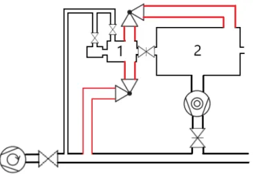
18 The insertion chamber is the one in which the transfer rod is inserted, as well as the one which allows introduction or removal of samples from the system. This chamber is fitted with a fast entry-lock system which allows easy mounting of samples on the fork with minimal leakage rates. When not transferring samples, this chamber is kept at 10-3 _{mbar range using a rotary} pump.

The preparation chamber was originally designed for different kinds of sample treatments such as thin film deposition or gas exposure. Connected to this chamber is a leak valve which allows introduction of different gases with high precision. This chamber also features a quadrupole residual gas analyzer (RGA) for chamber gas analysis and a XYZθ sample manipulator to move the sample as needed. A turbomolecular pump backed by the previously mentioned rotary pump is used to maintain the chamber at low 10-8 _mbar.

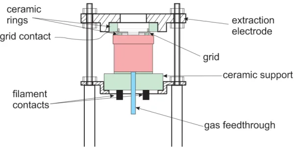
In order to simulate the conditions of a typical ionization gauge, a setup comprised of a tungsten filament, a positively biased tungsten grid and the extractor electrode, which hereafter will be referred to as the Ionization Gauge Simulator (IGS), was previously developed and mounted on this chamber. The schematic of IGS is presented in Figure 4.2. The design of IGS is based on that of electron impact ion sources. The latter is practically the same as the ionizer of residual gas analyzers (cf. Section 2.3) and similar to BA IGs. Electrodes are electrically separated using insulating pieces made of alumina (Al2O3). Beneath there is a hole through which gas can enter the IGS.

Figure 4.2: Schematic of the Ionization Gauge Simulator.

19 inaccurate and, as such, it was only used to expose the samples to IG-like conditions. During the exposure, the sample is situated ~ 3 mm below the top end of the extractor electrode, which secures uniform irradiation of the sample surface (of circular shape with ~12 mm in diameter) by different charged and neutral species leaving IGS.

The analysis chamber is used for the surface cleaning and analyses (XPS, IISEY and work function change). It encompasses an ion sputter gun, a movable filament used for the sample annealing by electron bombardment, a sample manipulator identical to the one in the preparation chamber and a carrousel in which the samples can be stored for later usage. This chamber also features an XPS system comprised of an X-ray source (either Mg or Al), a hemispherical energy analyzer working in the Fixed Analyzer Transmission (FAT) mode and a set of three channeltrons with an associated preamplifier. The preamplifier is comprised of a set of three identical circuits which were responsible for the amplification, noise filtration and TTL pulse formation of the signal provided by a single channeltron. These signals are then transferred to the computer acquisition board using Line Driver/Receiver pairs. The channeltrons are mounted in such way that one of them is positioned directly between the analyzer electrodes, with the remaining channeltrons being positioned on opposing sides equally shifted from the central channeltron. This means that electrons reaching the side channeltrons will have slightly shifted energy in respect to the central one. A homemade acquisition program allows energy correction, shifting the spectra of the side channeltrons signal and subsequent sum of all three signals [30]. The high voltages required to operate the decelerating lens system and the hemispherical analyzer are produced using a set of computer-controlled sources. High voltage is produced using a cascade voltage multiplier which converts small AC voltages into higher DC voltages. These voltages are proportional to the analog control voltage provided by the computer, which allows simple voltage regulation. All analyzer voltages are a result of a voltage division of a single source. Channeltron voltages are operated on a similar principle with the difference that the voltage regulation is performed manually through the usage of built-in potentiometers.

Since several sensitive techniques are performed in this chamber it is pumped with a combination of a 270 l/s ion pump and a titanium sublimation pump, which provide base pressure in the low 10-10 _{mbar range after proper baking.}

4.2. Repairs and improvements of the existing setup

20 improvements resulted in a system having considerably better abilities with respect to the initial ones.

4.2.1. Reconstruction of the fast entry lock pumping system

Initially, the introduction chamber was pumped via a tube having a quarter inch diameter, which had to be improved. Once the introduction chamber is pumped down, a gate valve connecting it to the preparation chamber is open in order to transfer the sample. This procedure was initially increasing the pressure in the preparation chamber for 3-4 orders of magnitude. Since the sample transfer in the analysis chamber cannot be safely performed before the pressure in the preparation chamber reaches at least 10-7 _{mbar range, the whole} procedure was lasting hours.

Figure 4.3: Introduction and Preparation chambers vacuum setup. Modifications are highlighted in red.

21

4.2.2. Reconstruction of the detection electronics

Low signal to noise ratio was the major problem of the whole system since the moment of its reassembling in the Laboratory. From time to time, the noise was even exceeding the true signal, which has been solved by changing the positions of different power supplies and of the cables connecting the preamplifier with the acquisition system. It should be noted that only one of the three preamplifier channels was able to work on an acceptable level. At the beginning of our experiments the noise problem became too much pronounced to be solved by pure improvisations. Therefore, the decision was made to identify the true source of noise and try to fix it.

While probing the system, several sources of instabilities were quickly identified, namely with the electron optics and channeltrons’ high voltage power supplies.

Regarding the optics power supplies, most of their problems were attributed to the contact issues. Some of these issues were fixed by simply cleaning the contacts, while the rest required rebuilding the connectors themselves. Furthermore, some of the power transistors were noticed to be unusually hot. These were consequently replaced due to the failure. Proper thermal contact was done to prevent further heating issues.

The channeltrons’ voltage source consists of two channels, with one of them being used to bias the inner and outer channeltrons and the other one being used to bias the remaining central channeltron. At the beginning of our experiments only one of these channels was working. While working on this unit, contact problems were identified pertaining to the

connector’s pins, which were loose therefore causing bad connection. After this issue was dealt with, a problem with the +15V supply voltage ripple filtering was identified. The unit was deemed faulty and swiftly replaced. At the end of the repairs, both high voltage channels were working as intended.

While these were definite improvements of the overall system, the main issue had yet to be resolved, namely the signal noise. The source of the noise was identified to be related to the preamplifier system. The noise problem was pinpointed to be related with the signal noise filtration after the first amplification stage. This part of the system used a differential comparator operational amplifier as a band-pass filter, which could be adjusted using a potentiometer located on the outside of the preamplifier. Through the usage of test signals, the problem was eventually discovered to be related to the band frequency being inadequate for the type of signal which the channeltron were providing. The pass band frequency is a function of the RC constant. With that in mind, the original 22 pF capacitors were replaced with 220 pF capacitors, therefore increasing the filtered frequency range. This provided an immense decrease in the previously observed noise.

22 others, and consequently decoupling the preamplifier channels. These resistors were increased to 10 MΩ (from the original 100kΩ) in order to allow higher precision of the band selection.

Several other changes were made with the goal of both further noise reduction in the system and prevention of eventual future problems. To start with, all the integrated circuits in the preamplifier were replaced with the pristine ones. The cabling to the acquisition board was repaired and proper shielding was made. While previously cabling positioning had to be constantly adjusted to avoid noise issues, it is no longer a contributing factor to the system noise. The acquisition box circuitry was also reworked by rearranging the cabling and removing ground loops which is a known source of noise. A faulty line receiver which was introducing noise to one of the acquisition channels was also replaced.

As a result of all these changes, all the preamplifier channels were made to work with acceptable noise (roughly 20-40 counts/s), which allowed much quicker and more reliable signal acquisition. As it currently stands, the detection system is substantially better than it ever was from the moment of the system purchase. Furthermore, all these changes lead to a better understanding of the system itself, which will prove helpful in solving future system malfunctions.

4.2.3. Design of the new acquisition system for the RGA

As a result of the repairs on the acquisition box, the board’s analog lines related to RGA were reconnected, returning it to a functional state. Previously developed Labview program was used for the processing and display of the RGA data. This program converts the analog

differential signal into integer values using Labview’s built-in functions. It then stores these values in an array and uses them to build a mass spectrum. This cycle is repeated until the user stops the acquisition.

The spectrum obtained through this method is inherently noisy. As a result, new code was implemented aiming to reduce the noise. The interface of the new software is shown in Figure 4.4. The method implemented consists of storing the data until the mass difference between the first and last stored measurement is equal or greater than the user defined range. These points are then averaged and used to build the new spectrum. A new range of points is then obtained and graphed until the final mass is reached. This process is done during acquisition.

23 Figure 4.4: RGA control software interface.

4.3. Experimental Procedures

The first step in this study involved choosing the materials for testing. From all the materials commonly used for electrode building, three were chosen: stainless steel (hereafter mentioned as SS), gold and molybdenum. Stainless steel was chosen because of its common use in all kinds of vacuum systems as well as its relative cheapness, with it being the first choice for collector composition of the new design which is being developed in the frame of the Empir project. Gold, on the other hand, is widely used as a coating in electrodes to minimize chemical reactions occurring at the electrodes themselves, so it is a material of interest in the project this study is part of. Molybdenum was one of the proposed materials, since it is widely used in ionization gauges. During the duration of the study, it became evident that some aspects of it had to be performed using highly pure samples. Towards that end, a single crystal copper sample was also tested. This sample was also used for XPS energy calibration using its Cu

2𝑝3/2 photoelectron and Cu L2M45M45 Auger lines as references.

24

foil samples were present in the analysis chamber and as such didn’t undergo manual

preparation. These were however sputter cleaned to remove the hydrocarbon layer which naturally develops with time on any surface. When not under the exposure, all samples remained deposited on the carrousel of the analysis chamber in order to preserve their surface conditions. Before the exposures, samples underwent several measurements.

The first of these was XPS analysis with the goal of finding the samples surface composition. During these measurements, XPS gun parameters were fixed to 10 mA of electron emission with 10 keV of acceleration. Two kinds of spectra were taken. The first one was a survey spectrum (low resolution) with the goal of the element identification and the peak location. This was done by scanning a broad section of the spectrum (from 0 eV to 600, for Au and Mo, or 1000 eV, for SS and Cu) with 0.5 eV energy steps lasting 0.5 seconds each in the FAT 40 mode (which means that analyzer pass energy is 40 eV). Following the peak identification, high resolution spectra was performed, which only scanned the elements’ main peaks. For the better resolution, these were performed with a 0.1 eV energy step lasting 4 seconds each, in the FAT 20 mode.

After the composition analysis, work function was measured by finding the cutoff energy (Ec) using the procedure described in the section 2.4. Lower X-Ray emission was used (1 mA of electron current with 5 keV anode voltage) alongside a narrowing of the analyzer’s entrance slit so as to reduce the number of electrons reaching the channeltrons, therefore increasing its work span, and increase the resolution. A small python script code was developed to accurately determine the energy cutoff from the secondary electron spectra data. This script works by finding the linear portion of the spectrum and fitting it to a first-degree polynomial, which is then used to find the intersection with the background level. The first 10 points are averaged to obtain an estimation of the background level. Following this, the program looks for maximum count rate and its correspondent energy position. It then looks for the points closest to 20% and 80% of the max count rate with lower energy than the peak (left side of the peak), using them to obtain a fitting linear equation. The energy cutoff is then analytically obtained by intercepting the fitted line with the background level.

25 Figure 4.5: IISEY measurement setup.

Following these measurements, the samples were transferred to the preparation chamber and placed underneath the IGS at a 3 mm distance from the extractor electrode (Figure 4.6). Argon was introduced using a precision leak valve, increasing the pressure from the low 10-8 _{mbar range to roughly} 9 × 10−6mbar. IGS’_{s filament current was gradually}

increased until 5 mA of electron emission was achieved, at which point the grid potential would be +200 V with respect to the filament, initializing the gas ionization and the exposure.

Exposures lasted for 15 minutes, with an average ion current measured on the sample of 500 nA.

26 Afterwards, the sample was put back in the analysis chamber, where XPS, WF and IISEY measurements were again performed.

27

5. Results

In this chapter the data obtained during this study are compiled. In it, the mass analysis of the gases used in the experiments were analyzed in detail followed by the composition analysis results of different samples. IISEY and work function changes are then compiled and correlated with the XPS data. Afterwards, studies were performed on the single crystal cooper sample with the goal of identifying the contaminants’ origin, as well as the results of the long-term exposure.

5.1. Mass Analysis of the gas in the IGS

Before studying the exposure effects, there is a need to know exactly what kind of particles will interact with the sample. To that end mass spectroscopy done using the RGA was performed while introducing Argon (Figure 5.1) and concentrated rotary pump residual gas (Figure 5.2). The residual gas was introduced in the IGS by connecting the corresponding gas line with the volume between the turbo-molecular and the rotary pump.

Figure 5.1: Mass spectrum of the gas after Argon introduction into the IGS.

H+

H₂+

F+

Ar+2

N2+, CO+

Ar+ 0 0.2 0.4 0.6 0.8 1 1.2

0 5 10 15 20 25 30 35 40 45

28 Figure 5.2: Mass spectrum of the gas after residual gas introduction in IGS.

As expected, the peak at mass 40, attributed to Ar+_{, is dominant in the mass spectrum} taken in the first case (see Figure 5.1). While the presence of typical residual gas constituents, namely hydrogen and probably CO, along with argon is not a surprise, this cannot be said for the peak at mass 19. At this point, the origin of this mass, attributed to fluorine, is an open issue. It is, however, well known that fluorine is a constitutive element of Viton, which can be found in the chamber in the form of UHV compatible gaskets.The existence of doubly ionized species (as seen on 5.1) provides valuable insight into the IISEY measurements. Having species of higher ionization states means that some ions will have particularly high potential energy. The latter will certainly affect IISEY. On the other hand, doubly charged ions will gain twice as much kinetic energy for the same extraction voltage, so that the kinetic emission may be happening at lower apparent energies than initially expected.

In the mass spectrum of the residual gas (the gas being pumped by the rotary pump) dominate water and its fragments (peaks at masses 1, 16, 17 and 18) along with nitrogen and oxygen. The ratio between N+ _{and O}+ _{peaks is close to the one in air (around 4:1), being a} fingerprint of a leak present in the gas line. However, this ratio is of about 5:1 for the N2+ and O2+ peaks, which indicate the presence of CO+.

Another point of interest is the degassing of the IGS electrodes due to heating of electrodes by the filament and/or ion and electron bombardment. Because of the IGS activity the highly energetic electrons that are produced can interact with the grid resulting in particle emission due to ESD. These particles can then be ionized and collected by the sample, being deposited on its surface. Mass analysis was performed to understand possible contaminants coming from the electrodes using the same parameters as during the exposures.

H+

H₂+

N+

O+

HOH+

N2+, CO+

O2+

0 0.2 0.4 0.6 0.8 1 1.2

0 5 10 15 20 25 30 35 40 45

29 Figure 5.3: Mass spectrum of the residual gas with IGS Off and On.

Figure 5.3 shows mass spectra of the gas in the preparation chamber with IGS on and off. One can see that under IGS usage the amount of CO+ _{and C}+ _{appeared, which is indicative} of the emission of hydrocarbons from the IGS. In addition, the peaks characteristic to water and hydrogen significantly increase. The later are expected surface impurities on the electrodes. Finally, one should note the appearance of the O2+ peak, probably indicating release of oxygen from surfaces covered with metallic oxides. To reduce the amounts of hydrocarbons emitted, the IGS was turned on during several hours so as to degas the electrodes. This procedure allowed some degree of reduction of the contamination. However, the electrodes were constantly being contaminated due to the sample introduction setup which meant that the process had to be redone periodically. Due to the time constrains and since the improvements were minor this was disregarded for the most part of the experiments. Fluorine peak can be also observed. This fluorine was speculated to come from Viton pieces that are located in the vicinity of the RGA. Due to the proximity to the filament, the Viton is degassed by heat. The intensity of the fluorine peak remained constant regardless of the IGS state. This is a confirmation of the previous speculation regarding its origin. Given the nature of this contamination its contribution

to the study can be neglected since the RGA wasn’t used during the sample exposure.

From this, several conclusions can be made regarding the exposure conditions. During the argon exposure, Ar+ _{and Ar}2+ _{will be the predominant ions bombarding the sample, while} residual gas would lead to a broader range of ions such as water fragments (HOH+_{, OH}+ _and O+_{) and nitrogen (N2}+ _{and N}+_{). Additionally, carbon species (CO}+ _{and C}+_{) are also expected to} collide with the sample surface independently of the gas used, although in lesser quantities. As

H+

H2+

C+ O+ OH+ HOH+ F+ CO+

O2+

0 0.2 0.4 0.6 0.8 1 1.2

0 5 10 15 20 25 30 35 40 45

30 for the exposure to the neutral species, water, hydrocarbon and oxygen molecules can be expected in the vicinity of the sample surface.

5.2. Influence of the material exposure to the IGS discharge on the surface

composition

This section is dedicated to the composition analysis of the proposed materials both before and after the exposure to the argon discharge.

5.2.1. Molybdenum

The spectrum taken from the molybdenum sample showed presence of three elements, namely Mo, C and O. The high-resolution spectrum of the Mo 3d line shows two Mo phases attributed to the metallic Mo (Mo 3d5/2 at 228.3 eV) and oxidized molybdenum (Mo 3d5/2 at 232.9 eV) [23]. This kind of XPS spectrum is typical for metallic surface long term exposed to air, when a thin oxide layer is formed on the top of a metallic bulk. The exact position of the oxide contribution MoOx undoubtable reveals that the dominant oxide phase is MoO3 [23]. Metallic oxide contribution was also detected in the O 1s line. A significant amount of carbon can also be detected. Carbon line is positioned at around 285 eV which is typical for hydrocarbon contamination (so-called adventitious carbon) [31]. Alongside this, oxidized carbon can also be observed due to the presence of C-O and C=O contributions in both C 1s and O 1s lines. This result clearly indicates that the Mo surface is covered with a layer of hydrocarbons, which also contains some amount of oxygen, a top the MoOx layer and the bulk metallic molybdenum.

31 contribution disappears after the sample exposure to the discharge. This means that the content of the hydrocarbon contamination due to the exposure is different from that due to the air exposure: the amount of carbon is more dominant in the latter case. It should be stressed that the drop of the C-O bonds is obvious from the change of the O 1s line shape as well.

Figure 5.4: Mo 3d5/3 line before the exposure to the Ar discharge. Name

Mo metal (3d 5/2) Mo metal (3d 3/2)

MoOx (3d 5/2) (+6)

MoOx (3d 3/2) (+6)

Pos. 228.296 231.496 232.932 236.015 %Area 45.12 30.08 14.88 9.92 1

x 102

8 10 12 14 16 18 20 22 c o u n ts p e r c h a n n e l

237 234 231 228

32 Figure 5.5: Mo 3d5/3 line after the exposure to the Ar discharge.

Having in mind low sputtering yield in the energy range used during the exposure (200 eV), significant drop of the MoOx phase intensity implies its small thickness. This is indeed the case, having in mind high surface sensitivity and the fact that we are getting considerable signal from the metallic bulk.

Name

Mo metal (3d 5/2) Mo metal (3d 3/2)

MoOx (3d 5/2) (+5)

MoOx (3d 3/2) (+5)

Pos. 228.329 231.429 231.717 234.817 %Area 47.33 31.55 12.67 8.45 1

x 102

8 10 12 14 16 18 20 22 c o u n ts p e r c h a n n e l

237 234 231 228

33 Figure 5.6: C 1s line before the exposure to the Ar discharge.

Figure 5.7: C 1s line after the exposure to the Ar discharge. Name C-C C-O C=O Pos. 285.011 286.411 288.612 %Area 65.01 24.05 10.94 x 101

120 130 140 150 160 170 180 190 c o u n ts p e r c h a n n e l

290 289 288 287 286 285 284 283

Binding Energy (eV)

Name C-C C-O Pos. 284.983 286.737 %Area 77.52 22.48 x 101

130 140 150 160 170 180 190 200 210 220 c o u n ts p e r c h a n n e l

289 288 287 286 285 284 283

34

5.2.2. Gold

Similarly, to the Mo sample, the survey spectrum of gold showed signs of C and O contamination, apart from the gold. Unlike Mo however, oxygen was purely organic in nature, which is expected due to the inert nature of gold. The main photoelectron line of Au, Au 4f, is shown in Figure 5.8. It contains a single contribution (Ag 4f7/2 at 84.0 eV), readily attributed to the metallic gold.

Figure 5.8: Au main peak.

After exposure to Argon discharge, the gold surface exhibited the same changes as the previous one: increase in carbon (6%) and oxygen reduction. The oxygen decrease rate is notably lower when compared with the Mo sample, which is to be expected since no oxide layer was present to be sputtered away.

5.2.3. Stainless Steel

Stainless steel analysis before the exposure revealed hydrocarbon contamination identical to the other samples. Although Fe and Cr peaks can be observed, they are small when compared with the more predominant C and O. This is to be expected, since the carbon and oxide layer screen the metallic bulk. Detailed analysis of the high-resolution spectra of Cr 2p3/2 and Fe 2p3/2 lines revealed the presence of metallic oxides, most likely CrO3 which makes up the protective oxide layer of SS, and organic oxygen.

Name

Au 4f 5/2 Au 4f 7/2

Pos. 83.9698 87.6198 %Area 57.14 42.86 1

x 102

30 40 50 60 70 80 c o u n ts p e r c h a n n e l

90 89 88 87 86 85 84 83 82 81

35 Figure 5.9: SS’s O 1s line before exposure.

Figure 5.10: SS’s O 1s line after exposure. 3rd block Name Metallic O C-OH O-C-O Pos. 530.035 531.605 533.418 %Area 29.40 50.83 19.77 2

x 102

22 24 26 28 30 32 34 36 c o u n ts p e r c h a n n e l

535 534 533 532 531 530 529 528

Binding Energy (eV)

Name Metallic O C-OH O-C-O Pos. 529.986 531.61 533.101 %Area 38.81 51.84 9.35 x 102

16 18 20 22 24 26 28 30 c o u n ts p e r c h a n n e l

535 534 533 532 531 530 529 528

36 Following exposure an increase in carbon (around 7%) was noted, with C-C becoming more predominant when compared with C-O bonds. As in the case of previous samples, the surface contamination during the exposure enhances the amount of saturated hydrocarbons (the relative amount of organic oxygen is decreased). The difference with respect to the Mo surface however appears concerning the metallic oxygen phase, which increased in intensity during the exposure. This can be observed when comparing the O 1s and Cr 2p3/2 lines taken before (Figures 5.9 and 5.11) and after (Figures 5.10 and 5.12) the exposure. Metallic and Cr2O3 contributions can be observed in Figures 5.11 and 5.12, but the oxide contribution increases with the exposure. Metallic contribution was fitted to an asymmetric line. That of Cr2O3, which has a complex shape due to the multiplet splitting effects, was fitted as a superposition of symmetrical peaks with well-defined constraints taken from the literature [21]. Comparison of both spectra seems to indicate a conversion of organic oxygen to metallic one. Given the predisposition of SS to spontaneously form a surface layer of Cr2O3, which prevents corrosion of this material, the result isn’t surprising. A decrease of the intensities of metallic contributions of both Fe and Cr corroborate with this general scenario. Interestingly, the overall amounts of Cr and Fe remained mostly unchanged throughout exposure.

Figure 5.11: SS’s Cr 2p3/2 line before exposure.

Name Cr2O3 Cr2O3 Cr2O3 Cr2O3 Cr2O3 Metallic Cr %Area 25.19 24.49 13.30 5.60 3.50 27.93 x 101

280 285 290 295 300 305 310 c o u n ts p e r c h a n n e l

580 579 578 577 576 575 574 573

37 Figure 5.12: SS’s Cr 2p3/2 line after exposure.

The results of the composition analysis before and after the exposure of the three samples are summarized in the Table 5.1. We clearly observe the same general trend: reduction of organic oxygen and additional contamination with saturated hydrocarbons. Having in mind that C is sputtered away alongside the oxide layers, it seems that parallel to the hydrocarbon layer being removed due to Ar sputtering, hydrocarbon contamination is occurring due to the IGS residual gas. In final, the net effect of the exposure to the IGS environment is additional contamination with saturated hydrocarbons.

Name Cr2O3 Cr2O3 Cr2O3 Cr2O3 Cr2O3 Metallic Cr %Area 30.93 30.06 16.33 6.87 4.30 11.52 x 101

230 240 250 260 270 280 c o u n ts p e r c h a n n e l

580 579 578 577 576 575 574

38 Table 5.1: Elemental quantification of the XPS spectrum for each sample.

Quantification [%]

Sample

Element

Before

Exposure

After

Exposure

Mo

Mo

11.75

13.39

C

48.89

59.49

O

39.36

27.12

Au

Au

15.51

13.24

C

68.60

74.33

O

15.89

12.43

SS

C

50.31

57.42

O

41.46

34.31

Cr

3.30

3.30

Fe

4.93

4.97

5.3. Influence of the Ar discharge exposure on the sample work function

Work function measurements reveal a slight shift in the emission threshold, in other words, a change in the sample’s work function. A shift of 0.10 eV, -0.25 eV and 0.38 eV were observed for molybdenum (Figure 4.13), gold (Figure 4.14) and stainless steel (Figure 4.15), respectively.

39 Figure 5.14: Au secondary electron spectrum.

Figure 5.15: SS secondary electron spectrum.