MISSING DATA IN TIME SERIES: ANALYSIS, MODELS
AND SOFTWARE APPLICATIONS
Francesca Minglino
Dissertationsubmitted as partial requirement for the conferral of Master in Management of Services and Technology
Supervisor:
Prof. José Dias Curto, ISCTE Business School, Departamento de Métodos Quantitativos para Gestão e Economia (DMQGE)
Supervisor:
Prof. Alberto Lombardo, Università degli Studi di Palermo, Dipartimento di Innovazione Industriale e Digitale
Spine example
-M
ISS
IN
G
D
A
T
A
I
N
T
IM
E
SE
R
IE
S:
A
N
A
L
Y
SI
S, MO
D
E
L
A
N
D
SO
FT
WA
R
E
A
PP
L
IC
A
T
IO
F
rance
sca
Mi
ngl
ino
A
BSTRACT
Missing data in univariate time series are a recurring problem causing bias and leading to inefficient analyses. Most existing statistical methods which address the missingness problem do not consider the characteristics of the time series when imputing the missing values and, most of all, do not allow the imputation in a univariate time series context. Moreover, just a few methods can be applied to all missing data patterns. Finally, no intuitive procedure addressing the missingness obstacle exists in the literature. In this work of investigation, an algorithm having the aim of filling in these gaps is presented; its main purpose is to find a procedure that gives reliable imputations of the missing values, i.e. not far from the true ones. To this aim, the reliability and robustness of the algorithm have been tested through the simulations campaigns approach. Its innovative feature is the combination of the ARMA models, used to impute the missing values through a forecast and a backcast approach, and the Expectation-Maximization algorithm, used to achieve the parameters convergence. This approach was evaluated through the RMSE and the MAPE metrics, which showed that the algorithm can be used in almost every model setting among the tested ones, with a good reliability. However, one of the main limitations of the introduced procedure is that the non-convergence of the algorithm could bring to biased imputations. The algorithm can be applied step by step by a common analyst, in a more intuitive way than the majority of other existing approaches.
Keywords: Missing Data; Univariate Time Series; ARMA Models; Expectation-Maximization
Algorithm.
I
NDEX
CHAPTER 1: INTRODUCTION ... 6
1.1OPPORTUNITY FOR INVESTIGATION ... 6
1.2OBJECTIVES OF THE RESEARCH ... 7
1.3RESEARCH QUESTIONS ... 8
1.4INVESTIGATION METHODOLOGY ... 8
1.5STRUCTURE OF THE THESIS ... 9
CHAPTER 2: LITERATURE REVIEW ... 10
2.1TIME SERIES ... 10 2.1.1 Components ... 11 2.1.2 ARIMA Models ... 12 2.2MISSING DATA ... 13 2.2.1 Patterns ... 15 2.2.2 Identification ... 17
2.3OLD METHODS TO HANDLE MISSING DATA... 17
2.3.1 Complete Case Analysis and Available Case Analysis ... 17
2.3.2 Single Imputation ... 18
2.4NEW METHODS TO HANDLE MISSING DATA ... 20
2.4.1 Maximum Likelihood Estimation and Expectation Maximization Algorithm ... 21
2.4.2 Multiple Imputation (MI) ... 23
2.4.3 Bootstrap ... 26
2.4.4 EMB Algorithm ... 28
2.4.5 Methods that deal with MNAR data ... 29
2.5SUMMARY OF THE LITERATURE REVIEW ... 31
CHAPTER 3: METHODOLOGY ... 33
3.1LITERATURE REVIEW ... 33
3.1.1 ARMA Models Definition ... 33
3.1.1.1 AutoRegressive Process of order p ... 33
3.1.1.2 Moving Average Process of order q ... 34
3.1.1.3 ARMA(p, q) Processes ... 34
3.2SIMULATIONS CAMPAIGNS ... 35
3.3ANALYSIS TOOL ... 36
CHAPTER 4: APPLICATION ... 37
4.1THEORETICAL APPLICATION ... 37
4.1.1 Time Series Simulation ... 37
4.1.2 Model Identification Step ... 39
4.1.3 Missing Data Simulation ... 39
4.1.4 Algorithm Implementation... 40
4.1.4.1 Algorithm Steps... 42
4.1.5 Assessment Metrics ... 43
4.2SOFTWARE APPLICATION ... 43
4.2.1 Time Series Simulation ... 44
4.2.2 Missing Data Simulation ... 44
4.2.3 Algorithm Implementation... 45
4.2.4 Assessment Metrics ... 48
4.3RESULTS AND DISCUSSION ... 48
4.3.1 Results Structure ... 48
4.3.2 Discussion ... 49
4.3.3 Results Summary ... 59
4.4VADEMECUM FOR THE USER ... 60
CHAPTER 5: CONCLUSIONS ... 63
5.1OVERVIEW ... 63
5.2ANSWER TO RESEARCH QUESTIONS ... 64
5.3CONTRIBUTION ... 66
5.4LIMITATIONS AND FURTHER INVESTIGATIONS... 67
REFERENCES ... 69
APPENDIX ... 72
1.ITERATIVE IMPUTATION STEP ... 72
1.1 AR(2) Process ... 72
1.2 MA(1) Process ... 72
1.3 MA(2) Process ... 73
1.5 ARMA(2,1) Process ... 75
1.6 ARMA(1,2) Process ... 75
1.7 ARMA(2,2) Process ... 76
ACRONYMS ... 77
F
IGURE
I
NDEX
FIGURE 1:DECOMPOSITION OF A TIME SERIES ... 12FIGURE 2:SCHEMATIC REPRESENTATION OF MULTIPLE IMPUTATION ... 23
FIGURE 3:BOOTSTRAP PROCEDURE IN A CONCEALMENT PROCESS ... 28
T
ABLE
I
NDEX
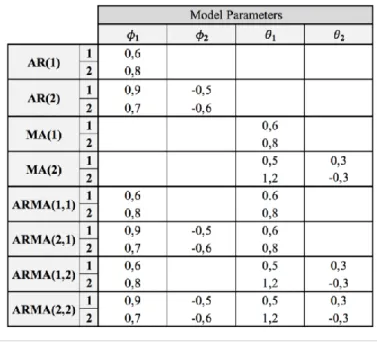
TABLE 1:PARAMETERS SETS FOR EACH ARMA MODEL ... 38TABLE 2:AR(1)MODEL SETTINGS RESULTS ... 50
TABLE 3:AR(2)MODEL SETTINGS RESULTS ... 50
TABLE 4:AR(2)MODEL SETTING WITHOUT NON-CONVERGENT SIMULATIONS ... 51
TABLE 5:AR(2)PROCESS SIMULATIONS EXAMPLE ... 51
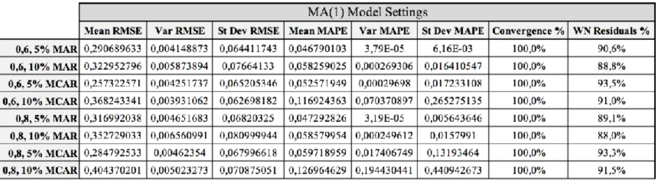
TABLE 6:MA(1)MODEL SETTINGS RESULTS ... 52
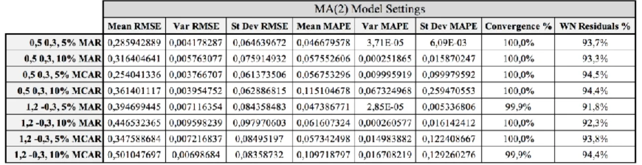
TABLE 7:MA(2)MODEL SETTINGS RESULTS ... 53
TABLE 8:MA(2)MODEL SETTINGS RESULTS WITHOUT NON-CONVERGENT SIMULATIONS ... 53
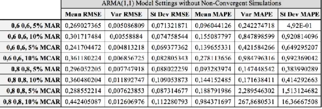
TABLE 9:ARMA(1,1)MODEL SETTINGS RESULTS ... 54
TABLE 10:ARMA(1,1)MODEL SETTINGS RESULTS WITHOUT NON-CONVERGENT SIMULATIONS ... 54
TABLE 11:ARMA(1,1)PROCESS SIMULATIONS EXAMPLE ... 54
TABLE 12:ARMA(2,1)MODEL SETTINGS RESULTS ... 55
TABLE 13:ARMA(2,1)MODEL SETTINGS RESULTS WITHOUT NON-CONVERGENT SIMULATIONS ... 56
TABLE 14:ARMA(1,2)MODEL SETTINGS RESULTS ... 56
TABLE 15:ARMA(1,2)MODEL SETTINGS RESULTS WITHOUT NON-CONVERGENT SIMULATIONS ... 57
TABLE 16:ARMA(1,2)PROCESS SIMULATION EXAMPLE... 57
TABLE 18:ARMA(2,2)MODEL SETTINGS RESULTS ... 58
TABLE 19:ARMA(2,2)MODEL SETTINGS RESULTS WITHOUT NON-CONVERGENT
C
HAPTER
1:
I
NTRODUCTION
Time series data can be found in nearly every study field, going from healthcare to finance, from social science to the energy industry. Many researches focused on time series analysis (Box and Jenkins, 1970; Chatfield, 2000; Brockwell and Davis, 2016) since these data show some features allowing to extract a lot of information about the process which generated them. Nearly everywhere, however, when data is measured and recorded, some issues linked to the missing values occur. Various reasons can lead to missing data: for instance, values may not be properly collected or measured, values could be measured by considered unusable by the analyst. Real life examples can be the closure of the markets for one day, the malfunction of the sensor recording some movements, a communication error (Moritz et al., 2015). Missing data can present different patterns and frequencies (Rubin, 1976) and their presence can lead to various problems. Indeed, when a missingness mechanism occurs, further data processing and analysis steps cannot be pursued since the common software statistics are not able to handle the missing data. Furthermore, the absence of data reduces the statistical power of the tests, which refers to the probability that the test will reject the null hypothesis when it is false, and can cause bias in the estimation of parameters. Moreover, also the representativeness of the chosen sample could be put in question. These are the main reasons why missing data have to be replaced with reasonable values, which do not have to bring sharp modifications to its distribution and the data generating process. A lot of researches have been done in this field in order to find trustworthy techniques to fill the missing values in without damaging the distributional shape of the data.
Many researches focused on different missing data imputation techniques, among which the most known ones are the Single and Multiple Imputation (Rubin, 1976; Rubin, 1987), as well as the Maximum Likelihood Estimation through the Expectation Maximization algorithm (Dempster et al., 1977), the Bootstrap (Efron, 1994) and also the Expectation-Maximization with Bootstrapping (EMB) algorithm (Honaker and King, 2010). The strength of the application of these kinds of solution to the problem of missingness is that the output is a complete dataset, ready to be analysed through all the basic and more sophisticated statistics.
1.1
O
PPORTUNITY FORI
NVESTIGATIONIn the context of the problem of the missing data in time series, in the existing literature only a limited number of researches have focused on the specific case of univariate time series
imputation. In fact, just a few software applications exist in this field. The imputation methods mentioned before are, indeed, thought to be applied to multivariate datasets. Specifically, in order to be applied to time series data, these methods have to be adapted to consider the interactions in time beyond those in space: the process generating a time series indeed shows its features over time, therefore the lagged values of a variable have their own weight in describing the following values (Box and Jenkins, 1970), together with the other variables’ present and lagged values if the dataset under analysis is a panel. Furthermore, in order to handle a univariate time series, the above-mentioned methods cannot rely on inter-variables interactions since just a time series is being considered. They must be adapted again in order to rely only on interactions over time of a time series own values. Therefore, univariate time series are a special challenge in the field of missing data imputation. It is reasonable to tailor the imputation algorithms in order to take into account both the characteristics of the time series and the lack of inter-variables interactions.
Another consideration has to be made, about the existing imputation algorithms. These methods are usually of low intuitiveness and of difficult implementation for a common user, who is dealing with the missing data problem for the first time. Moreover, even to employ one of the few existing software applications to bypass the problem of the missing data, a common user has to study part of the literature about the topic to understand what the software is doing and how to interpret the output.
The combination of these two gaps in the state of the art, which are the few researches about the univariate time series with missing data scenarios and the need of a guided software implementation, represent the opportunity to start this investigation.
1.2
O
BJECTIVES OF THER
ESEARCHThe general aim of this dissertation is to build an intuitive guided software application for dealing with missing data in a univariate time series scenario. The idea of the guided application is that the user, following the procedure step by step, could be able to handle his/her missingness problem without the need of looking for an explanation elsewhere. Further, the algorithm on which the application is built has to rely on basic time series concepts in order to be widely used and understood by the common users. Of course, the algorithm should give back reliable results, that the analyst can use to his/her own purpose.
1)Time Series Data Structure
1.1) Identify the principal aspects to be included in a time series analysis; 1.2) Identify the most widely used models to fit a time series;
1.3) Define the impact of the missingness on time series data.
2)Missing Data Imputation Methods
2.1) Analyse the principal objectives of the application of an imputation method; 2.2) Identify the requirements of univariate time series analysis;
2.3) Build a procedure based on the previous objectives’ development;
2.4) Determine how to sketch the built procedure to meet the user’s intuitiveness needed.
1.3
R
ESEARCHQ
UESTIONSStarting from the specific objectives of the research, with the final aim to meet the general objectives explained in the previous paragraph, this dissertation will answer to the following research questions:
1)Time Series Data Structure
Q1: “Is it possible to preserve the process generating a univariate time series
when missing data occur?”
2)Missing Data Imputation Methods
Q2: “Is it possible to apply the same imputation algorithm structure to any
missingness case?”
Q3: “Is it possible to apply the same imputation algorithm structure to both
univariate and multivariate time series scenarios?”
1.4
I
NVESTIGATIONM
ETHODOLOGYThis investigation started in October 2017 and finished in September 2018. The purpose of this exploratory work is to give a contribution to the research field of the univariate time series with missing data.
The investigation methodology applied in this work follows an inductive approach. The research started from the literature review, which brought to the identification of the main topics associated to the time series with missing data and to the definition of the propositions that were used in the work. After this step, the application of a method built on the basis of the already existing approaches was done on simulated data. Furthermore, the results of the application of the procedure were analysed in order to assess the goodness-of-fit of the method. The final step
of the investigation was the definition of a vademecum about the whole methodology to be applied in this kind of situations.
1.5
S
TRUCTURE OF THET
HESISThis work is organized in five chapters. Chapter 1 is the introduction, which explains the objectives of the investigation, as well as the research questions. In Chapter 2, the literature review is developed, divided in 5 Sections: in the first one the Time Series Data are described; in the second one the problem of the Missing Data is introduced, with an insight about the patterns they can follow; the third and fourth sections deal with the old and new methods (respectively) used to handle the missingness problem; in the fifth and final section, a summary of the literature and the definition of the propositions is done. Chapter 3 deals with the description of the methodology applied. In Chapter 4 the application of the method is shown, with an overview about the code used in the software R, the statistical analysis tool. In the same chapter, the results of the application are presented and discussed and the vademecum built for the users is shown. Finally, Chapter 5 presents the conclusions, in which an answer to the research questions is given and the contribution of the work is reported. In the same final chapter, also the limitations and the starting points for further research are explained.
C
HAPTER
2:
L
ITERATURE
R
EVIEW
The aim of the literature review is to collect, analyse and resume in a critical way the existing literature about the topic being studied, identifying the theories and studies underlying it in an integrated form. Thanks to the literature review, it was possible to identify the gap whose solution is the aim of this study. This chapter is divided in five main parts: in the first one, an overview about time series, its characteristics and the ARMA models is done; the second part is dedicated to the Missing Data, therefore the problem arising with the missingness is explained, as well as the different patterns they can show; in the third part, the old models used to handle the missingness in a variable or a set of variables are analysed, highlighting the advantages and the limitations; in the fourth part, the new and more sophisticated models are analysed and compared. Finally, a summary of the most important findings from the literature analysed is composed.
Because of the complexity of the investigation topic, in this literature review, before even highlighting strengths and weaknesses, the description of the features and of the application of each method is introduced. This choice was made to give to the reader an overview about the differences among the existing methods, in order to focus afterwards on the conditions under which a method can be preferred to another one.
2.1
T
IMES
ERIESA discrete time series is a sequence of discrete-time data, taken at successive equally spaced points in time. Data in time series present some interesting features, useful for conducing statistical analysis whose aim is to extract information about the observed phenomenon and to forecast the next values that the series can present. For instance, assuming that the variable Yt
has been generated by a stochastic process, it is common to find a link between the variable at time t and its lagged values Yt-1, Yt-2, …, Yt-j. For this reason, the past observations of a variable
can be used to say something about their generating process.
A time series yt can be regarded as a particular realization of a stochastic process Yy (Brockwell
and Davis, 2016) and so it presents a mean (𝜇𝑡), a variance ( 𝜎𝑡2) and a covariance (𝛾
(𝑡,𝑠)) when
they exist) defined as follows:
E(Yt) = 𝜇𝑡 t = 1, 2, … , T
V(Yt) = E(Yt-𝜇𝑡)2 = 𝜎𝑡2 t = 1, 2, … , T
When these moments are independent of t, the series is said to be stationary. If it is not, some transformations like the first difference and/or the logarithm have to be applied in order to obtain a stationary series. Usually, those are sufficient to this aim. In this work, heteroskedasticity issues are not taken into consideration: the conditional variance of the errors will be always assumed as constant. So, just homoskedastic time series will be considered in this investigation. Further studies could focus on this issue.
In the following paragraphs, the variations that a time series can present over time and some models dealing with stationary processes are treated.
2.1.1
C
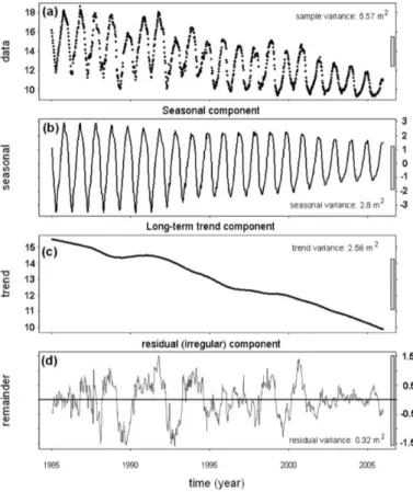
OMPONENTSA time series is rarely perfectly constant over time. Indeed, it usually presents some variations, and it can be decomposed in four components which may or may not exist at the same time. The components are:
1. Seasonal variation. This type of variation refers to cycles that repeat regularly over time, generally annually. It arises for many series, whether measured weekly, monthly or quarterly, when similar patterns of behaviour are observed at particular times of the year (Chatfield, 2000). An example are the retail sales, which tend to peak for the Christmas season and then decline after the holidays;
2. Trend. This type of variation is present when a series exhibits a growth or a decrease over time. It can be defined as a long-term change in the mean level. A time series can present a stochastic or deterministic trend, which can be linear, as well as quadratic, parabolic or any other shape. The trend is usually the result of long-term factors influence like changes in demographics, technology or customers habits;
3. Cyclical variation. This variation includes a cyclical variation which does not present regular repetitions over time and lasts more than one year. It is usually hard to estimate, since the distance in time between two cycles can be long and it is not constant. Examples include business cycles over periods of five or more years and the periodic variations in nature, for instance regarding temperature or the lifecycle of the beings;
4. Irregular fluctuations. This last variation is the part of the time series which has been ‘left over’ after trend, seasonality and other systematic effects have been removed. The irregular component of a time series is unpredictable, since it may be completely random. The irregular component catches also sudden variations such as an increase in the price of steel due to a strike in the factory, reflecting some extraordinary events.
The Figure 1 below shows graphically how a raw time series can be decomposed in its components, in the case in which it presents them all. Since the cyclical variations are hard to detect, the decomposition models include this component into the trend.
Figure 1: Decomposition of a time series
2.1.2
ARIMA
M
ODELSThe ARIMA class of models is an important forecasting and time series analysis tool. These models are also known as the Box-Jenkins models since these two authors first introduced a method for implement them in an efficient algorithm. The acronym ARIMA stands for ‘AutoRegressive Integrated Moving Average’, where the Integrated part indicates the number of differences needed to turn the series into stationary. The other two components, the AutoRegressive and the Moving Average indicate whether the observation at time t depends on its lagged observations or on the previous shocks (errors), or on both. In an ARIMA(p, d, q) model, the letters p and q state the maximum lag order still influencing the variable at time t, respectively for AR(p) processes and MA(q) processes. Finally, the letter d regards the integrated part, as it was said previously.
In this work, as will be explained more in detail in Section 4.1.1, only stationary time series will be considered. Therefore, from now on, the ARIMA(p, 0, q) models, that can be written in the equivalent form ARMA(p, q), will be employed.
In order to set an ARMA model in a proper way, it is suggested to have more than 100 observations for each time series, although this could increase the cost of data collection. Despite the high number of observations needed, the ARMA models catch the behaviour of the time series in a better way in the short run (Box and Jenkins, 1970) and this is the main advantage in employing this class of models. Moreover, while building a proper time series model, the principle of parameters parsimony has to be considered. The Box-Jenkins models follow this principle and favour the one with the smallest possible number of parameters out of a number of suitable models. The simplest one, that still maintains an accurate description of inherent properties of the time series, is preferred to the more complex ones. Box and Jenkins (1970) introduced as main scope of the ARMA models the identification and the estimation of the model underlying a time series, with the final aim to perform a forecast of one or more future data. However, through the same identified and estimated model, also a back-forecast (or backcast) can be applied in order to find older values than the observed time series. The ARMA models represent the more flexible and easier to adapt approach to the time series analysis and it is the reason why this investigation prefers the application of this class of models rather than, for instance, the smoothing models one.
In Section 3.1.1, further details about the ARMA models applied in this investigation is presented.
2.2
M
ISSINGD
ATAIn statistics, when no data value is stored for the variable in an observation, a missing datum or value occurs. Missing data are common in research in economics, sociology, and political science when governments choose not to, or fail to, report critical statistics. Sometimes, also data collection can cause missing values when, for instance, the researcher mistakes in data entry or collects the responses unproperly. Rubin (1976), for instance, introduces his paper presenting the problem of surveys addressed to families, which could not be located in the following years to repeat the same survey. Situations like this one create missing values. When missing data are found in a time series, this causes a lot of troubles. Indeed, since the special feature of time-series data is that consecutive observations are usually not independent and so the order in which the observations are collected has to be taken into account, when a missingness occurs the analysis of the following observations becomes harder due to the lack of precious information.
1.Description. Describing the data using summary statistics and/or graphical methods is difficult since the most part of software statistics do not work when a time series presents missing data. A time plot of the data would show holes in the series;
2. Modelling. Finding a suitable statistical model to describe the data-generating process, based only on past values of that variable considered, loses power if some observations are unhelpful to this scope. The statistical model found could be different from the real one;
3. Forecasting. As a consequence of the previous two steps, forecasting the future values of the series presents biases and low efficiency, due to the difficulties in describing and modelling the series.
Summarizing what said, the goal of a statistical procedure should be to make valid and efficient inferences about a population of interest in order to use the extracted information to various aims. When looking for a way to find a value as close as possible to the missing one, some considerations have to be made to avoid damaging the inferences about the entire population. Let’s consider for instance the easiest way to fill in the missing data, i.e. the common practice of mean substitution. The method consists in replacing each missing value with the mean of the observed values. This may accurately predict missing data but distort estimated variances and correlations (Shafer and Graham, 2002). A missing value treatment is embedded in the modelling, estimation, or testing procedure applied to the whole-time series and basic criteria for evaluating statistical procedures have been established by Neyman and Pearson (1933). For instance, let’s assume that 𝑄 denotes a generic population quantity (parameter) to be estimated and that 𝑄̂ is an estimate of 𝑄 based on a sample of data. If the sample includes missing values, then the method that will be used to handle them should be considered part of the overall procedure for calculating 𝑄̂ . If the whole procedure works well, then 𝑄̂ will be close to 𝑄 (Shafer and Graham, 2002), therefore showing small bias and standard deviation. Bias and variance are often combined into a single measure called mean square error (MSE), which is the average value of the squared distance (𝑄̂ − 𝑄)2 over repeated samples. However, even if
the procedure gives a low MSE as output, one should avoid solutions that apparently solve the missing data problem but actually redefine the parameters or the population. For instance, the mean substitution gives a biased estimation of the variance of the process since the estimate is lower than it should be. This effect should be always controlled by the analyst.
2.2.1
P
ATTERNSGoing more in depth in the analysis of the missing data in a time series, survey methodologists have historically distinguished unit nonresponse from item nonresponse (Lesser and Kalsbeek, 1992): the first one occurs when the entire data collection procedure fails (for instance because the sampled person is not at home or refuses to participate, etc.) while the second one occurs when partial data are available (for instance the participant does not respond to certain individual items). In this work, only item nonresponses are analysed.
The missingness of the data can be related to the observed data, can be caused by a random process or can be linked to some specific reasons. Adopting the generic notation introduced by Rubin (1976), but adapting it to the time series domain, let’s imagine a complete time series
𝑌𝑡 𝑐𝑜𝑚, which can be partitioned in the observed part 𝑌𝑡 𝑜𝑏𝑠 and in the missing part 𝑌𝑡 𝑚𝑖𝑠 such
that 𝑌𝑡 𝑐𝑜𝑚 = (𝑌𝑡 𝑜𝑏𝑠, 𝑌𝑡 𝑚𝑖𝑠). Let’s assume M as the missingness vector, which takes the value 0 if the datum is observed and 1 if it is missing. Rubin (1976) defined missing data to be Missing At Random (MAR) if the distribution of missingness does not depend on the missing data 𝑌𝑡 𝑚𝑖𝑠
such that
𝑃(𝑀 𝑌⁄ 𝑡 𝑐𝑜𝑚 ) = 𝑃(𝑀 𝑌⁄ 𝑡 𝑜𝑏𝑠 ) (1)
MAR means there is a systematic relationship between the propensity of missing values and the observed data, but not the missing data. Whether an observation is missing has nothing to do with the missing values, but it does have to do with the values of an individual’s observed variables.
A special case of MAR occurs when the distribution of the missing data does not depend on
𝑌𝑡 𝑜𝑏𝑠 either. This case is defined Missing Completely At Random (MCAR) and it can be
explained as
𝑃(𝑀 𝑌⁄ 𝑡 𝑐𝑜𝑚 ) = 𝑃(𝑀 ) (2)
MCAR, means there is no relationship between the missingness of the data and any values, observed or missing. The missing data points are a random subset of the data. There is nothing systematic going on that makes some data more likely to be missing than others. MAR and MCAR are both considered ignorable because no information about the missing data itself has to be included when dealing with the missing data. Instead, the third pattern of missingness that could occur is called non-ignorable, since the missing data mechanism itself has to be modelled. This is the case of Missing Not At Random (MNAR) data, when there is a relationship between the propensity of a value to be missing and its own values. In this last
case, some model to explain the missingness has to be included. It is the most difficult situation to deal with.
Notice that Rubin (1976) definitions describe statistical relationships between the data and the missingness, not causal relationships.
The assumption of MCAR data is usually very strong to hold. For this reason, in most of the cases, the assumption of the analysts is MAR. However, using maximum likelihood procedures as explained in the following paragraphs, one may achieve good performances without being sure about the distribution of missingness.
Assuming that 𝑌𝑡 𝑐𝑜𝑚 comes from a population distribution 𝑃(𝑌𝑡 𝑐𝑜𝑚; 𝜃), where 𝜃 is the set of
𝑌𝑡 𝑐𝑜𝑚 parameters (which can be the ARMA ones), it is tempting to ignore the missing data and
base all the statistical analysis on the distribution of the observed portion of data 𝑃(𝑌𝑡 𝑜𝑏𝑠; 𝜃)
(Shafer and Graham, 2002). This distribution could be obtained as
𝑃(𝑌𝑡 𝑜𝑏𝑠; 𝜃) = ∫ 𝑃(𝑌𝑡 𝑐𝑜𝑚; 𝜃) 𝑑𝑌𝑡 𝑚𝑖𝑠 (3)
as explained in Hogg and Tanis (1997) texts on probability theory. As Rubin (1976) explained, however, using this equation as base for the statistical procedures is not always correct, since it represents a proper sampling distribution for 𝑌𝑡 𝑜𝑏𝑠 only if missing data are MCAR and it is a correct likelihood if data are at least MAR. If data cannot be considered MAR, a distribution for M has to be chosen, since it would be the case of non-ignorable missingness. Let 𝑃(𝑀 𝑌⁄ 𝑡 𝑐𝑜𝑚; 𝜉) be a model for M, where 𝜉 is the set of parameters of the missingness distribution. The joint model for the whole set of data would depend both on 𝜃 and on 𝜉 as follows
𝑃(𝑌𝑡 𝑜𝑏𝑠, 𝑀; 𝜃, 𝜉) = ∫ 𝑃(𝑌𝑡 𝑐𝑜𝑚; 𝜃) 𝑃(𝑀 𝑌⁄ 𝑡 𝑐𝑜𝑚 ; 𝜉) 𝑑𝑌𝑡 𝑚𝑖𝑠 (4)
The practical implication of MNAR is that the likelihood for 𝜃 now depends on an explicit model for M. Many restrictions and limits occur when dealing with unknown patterns of missing data. For this reason, it is important to find models that do not need strict assumptions about the missingness pattern, unless one is able to correctly identify the distribution of the missing data, and to try to use the whole dataset. Especially when the series is a time series, every observation has its own weight and omitting some values can bias the estimates of the parameters of the whole distribution.
2.2.2
I
DENTIFICATIONThere is no exact science about how to identify the pattern of missingness. Some empirical analysis however can be done by the analyst before starting the process of imputation of the missing values. The only way to distinguish between MAR and MNAR is to try to measure some of the missing values by asking the non-respondent to answer to some key survey items. This could mean also asking them the reason why they didn’t answer. However, in most missing data situations, it is rare to have the possibility to directly speaking with the non-respondents. So, the most used practice is to analyse the type of data and try to get a conclusion. For instance, if the series regards the aggregate consumption of cocaine in the last 20 years and some of the data are missing, it is more likely that data are MNAR than MAR since people could not be willing to declare the number of grams of cocaine they consume. Or, if measuring the body pressure of an individual, values are less likely to be written down if the previous day observation is higher than 160, then data are more likely to be MAR instead of MNAR. Distinguishing from MAR and MCAR is more difficult in a univariate scenario than in a multivariate one. Indeed, for multivariate datasets it is possible to apply the Little test (Little, 1988) or also another R package called MissMech (Jamshidian et al., 2014). Further studies about this topic have been done by Heitjan and Basu (1996) and, apart from evidencing the differences in the behavior of the results if data were MAR or MCAR, they highlighted that these two patterns of missingness still let the analysts to work with that dataset. For this reason, the two patterns are called “ignorable”.
To conclude, what an analyst can easily do to continue his/her studies is to assume a pattern basing the assumption on his/her own experience about the data field or about the context of data collection.
2.3
O
LDM
ETHODS TO HANDLEM
ISSINGD
ATAIn this section, the Old Methods to deal with the missing data are explained. The most known ones are the Complete Case Analysis, the Available Case Analysis and the Single Imputation.
2.3.1
C
OMPLETEC
ASEA
NALYSIS ANDA
VAILABLEC
ASEA
NALYSISThe Complete Case Analysis, also known as Listwise Deletion, confines attention only to units that have observed values for all variables under consideration. Therefore, the method omits the missing data from the analysis, as if they had never been included among the observed values. This procedure does not give biased results only when data are MCAR. When the missing data are not MCAR, results from listwise deletion may be biased, because the complete
cases could be unrepresentative of the full population. If the departures from MCAR are not huge, then the impact of this bias might be unimportant, but in practice it can be difficult to judge how large these departures might be. Little and Rubin (1987) suggest to reduce biases from listwise deletion in some non-MCAR scenarios by applying weights to the considered observations so that their distribution is closer to the full population one. The only difficulty in this procedure is to find the right weights from the probabilities of responses, which is not always easy and unbiased.
Clearly, even if Listwise Deletion could give unbiased results if data are MCAR, when this method is applied to a time series more problems occur. For instance, if the observation interval is a month and a time series has 12 observations per year, eliminating one of these values because it is missing implies to slip one month forward the previous month observation (March observation is missing and it is deleted, February observation takes its place). No more seasonality studies can be made on this time series. For this reason, Complete Case Analysis won’t be taken into consideration in this study.
Available-Case (AC) Analysis, in contrast to the Complete Case Analysis, only considers different sets of sample units for different parameters. This means that, without deleting any value, parameters are estimated from different sets of units, probably of different length. As regards to a time series for instance, if it presents 20 consecutive observed values, then a missing one, then other 10 consecutive observed values, one could estimate an ARIMA model splitting the series so to only consider the two strings of observed data. Of course, this procedure leads to difficulties in computing standard errors or other measures of uncertainty. The estimated parameters of the series could be very different among them and also from the original series parameters. Although Kim and Curry (1977) argue that the Available Case Analysis can improve the quality of the estimates if compared to the Complete Case Analysis, other studies (Little and Rubin, 1987; Little, 1992) do not agree with that. To conclude, also the Available Case Analysis won’t be used in this work since the uncertainty about the parameters resulting from the analysis is too high to be handled.
2.3.2
S
INGLEI
MPUTATIONSingle Imputation is a simple method introduced by Rubin (1987) which involves filling in a value for each missing value. This method presents two main features of interest, which turn it more attractive than the listwise deletion. First, after imputing the missing values, standard complete-data methods of analysis can be run on the complete series. As a consequence, dealing
with complete datasets allows all kinds of users to reach reasonable conclusions about the data being analysed, applying the statistical tools they already know in any dataset. Second, imputations can incorporate the data collector's knowledge which, in many cases involves better information and understanding of the process being studied. The data collector could also know the possible reasons creating nonresponses.
Single Imputation is potentially more efficient than complete case analysis because no units are omitted. The retention of the full sample helps to prevent loss of power resulting from a diminished sample size (Shafer and Graham, 2002). Moreover, if the observed data contain useful information for predicting the missing values, an imputation procedure can make use of it and maintain high precision. Indeed, if a time series presents trend and/or seasonality, this information can be used to impute a value closer to the real one.
Single Imputation however presents also some disadvantages: indeed, a single imputed value cannot consider the uncertainty due to the unknown missing value and the uncertainty due the imputation model itself. This can lead to underestimate the consequences of these two uncertainties, such as a too optimistic variance.
For instance, considering a Single Imputation model of mean substitution, this could impute reasonable values for the ones which were missing, since the best prediction of a sample of data is its own mean, but it gives back a too small variance. Indeed, the mean is calculated on the
nobs observed values of 𝑌𝑡, instead of on the n total values. After imputing the missing values
by substituting the mean of 𝑌𝑜𝑏𝑠, the variance of the whole series turns to be smaller than it should, by a factor of 𝑛𝑜𝑏𝑠
𝑛 . This leads also to excessively large significance levels: this means
that the estimated variance is biased.
It is generally more desirable to preserve the distribution of a variable. Survey methodologists, field in which nonresponses are common, have developed a wide array of single-imputation methods that more effectively preserve distributional shape (Madow, Nisselson, & Olkin, 1983). For instance, one of the procedures is the hot deck imputation which, in the case of univariate replaces each missing value by a random draw from the observed values. However, this method still distorts correlations and other measures of association. Both mean substitution and hot deck produce biased estimates for many parameters under any type of missingness. Another type of single imputation is the one based on conditional distribution which, under MAR assumptions, produces nearly unbiased estimates. Supposed that 𝑦𝑡 𝑐𝑜𝑚, where 𝑦𝑡 𝑐𝑜𝑚 =
(𝑦𝑡 𝑜𝑏𝑠, 𝑦𝑡 𝑚𝑖𝑠) , comes from the distribution 𝑃(𝑌𝑡 𝑐𝑜𝑚; 𝜃) , imputing from the conditional
𝑃(𝑌𝑡 𝑚𝑖𝑠⁄𝑌𝑡 𝑜𝑏𝑠; 𝜃) = 𝑃(𝑌𝑡 𝑜𝑏𝑠, 𝑌𝑡 𝑚𝑖𝑠; 𝜃)
𝑃(𝑌𝑡 𝑜𝑏𝑠; 𝜃) (5)
where 𝜃 is actually 𝜃̂, the estimator of 𝜃 obtained from 𝑦𝑡 𝑜𝑏𝑠 (Schafer and Graham, 2002).
One application of the single imputation through the conditional distribution in the field of the time series is given by Kihoro et al. (2013). The idea of their procedure was to put together the ARIMA process followed by a time series with an iterative imputation method. The researchers, after having identified the ARIMA/SARIMA model which seemed to fit better with the series, estimated the parameters of the observed part of the variable. Through these parameters estimates, the first missing value was then filled in. The following step was to estimate again the parameters of the series, considering also the filled-in value, so to be able to fill in the second missing value and so on. Making an example, let’s consider a time series yt, presenting
𝑚 = 𝑚1, … , 𝑚 missing data and following ARMA(1,1) process. The parameters to be estimated are therefore 𝜃1 and 𝜑1, from the observed part of the data 𝑦𝑡 𝑜𝑏𝑠. After estimating the two parameters, the first missing value 𝑦𝑚1 is imputed as 𝑦𝑚1 = 𝜃1𝑦𝑚1−1+ 𝜑1𝑒𝑚1−1. The
parameters are estimated again including the imputed value of 𝑦𝑚1. 𝑦𝑚2 is then imputed in the same way and the entire procedure ends when all the missing values are filled in.
Even if the method considers the process underlying the series, the simulations the researchers did to test the effectiveness of this procedure did not provide quite good results.
In the context of a time series, the most part of single imputation methods are not able to take into account the relationship existing among the data: if the time series is an autoregressive process, replacing a missing value with a random draw from the rest of the data does not reflect the nature of the variable. If replacing the missing value with the mean, the information about eventual trend or seasonality would be lost. Drawing from the conditional distribution as in the study of Kihoro et al. (2013) could instead preserve the nature of the time series but some modifications have to be made in order to reach better results.
To conclude, although the intuitive easiness of the single imputation class of methods, the defect of underestimating variability and of losing precious information about the nature of the time series is insurmountable and this is the reason why other more precise methods are usually preferred.
2.4
N
EWM
ETHODS TO HANDLEM
ISSINGD
ATAA good missing data handling technique to has to satisfy three requirements: • it should allow standard complete-data methods to be used;
• it should yield valid inferences that produce estimates and standard errors that reflect the reduced sample size as well as the adjustment for the observed-missing values differences;
• it should display the sensitivity of inferences to various plausible models for missingness. The new methods to handle the missingness in a dataset try to achieve these requirements, that is the reason why they are usually preferred to the old ones. In this Section, the Maximum Likelihood Estimation with the Expectation-Maximization Algorithm, the Multiple Imputation, the Bootstrap and the EMB Algorithm are discussed.
2.4.1
M
AXIMUML
IKELIHOODE
STIMATION ANDE
XPECTATIONM
AXIMIZATIONA
LGORITHMThe Maximum Likelihood can be used to estimate the parameters of a variable although the presence of missing data. Literature shows that this method gives good results and, most of all, can be used with any missing data pattern. A general optimization algorithm for ML in missing data problems was described by Dempster et al. (1977) in their influential article on the Expectation-Maximization (EM) algorithm. This brings the ML, together with the EM, to be widely used. In order to have an insight about how the ML works, let 𝑦𝑡 𝑐𝑜𝑚 denote a time series, decomposed as before in its two parts, the observed and the missing one such that
𝑦𝑡 𝑐𝑜𝑚 = (𝑦𝑡 𝑜𝑏𝑠, 𝑦𝑡 𝑚𝑖𝑠) . Being Equation (3) the marginal probability density of 𝑌𝑡 𝑜𝑏𝑠,
assuming that the missing data mechanism could be ignored, Little and Rubin (1987) defined the likelihood of 𝜃 as any function of 𝜃 proportional to P(𝑌𝑡 𝑜𝑏𝑠⁄ ) as follows 𝜃
𝐿𝑖𝑔𝑛(𝜃 𝑦⁄ 𝑡 𝑜𝑏𝑠) ∝ 𝑃(𝑌𝑡 𝑜𝑏𝑠⁄ ) 𝜃 (6)
When the missing data mechanism cannot be ignored (MNAR data) however, the distribution
of 𝑦𝑡 𝑜𝑏𝑠 becomes as in Equation (4) and so the likelihood function of 𝜃 becomes
𝐿(𝜃, 𝜉 𝑦⁄ 𝑡 𝑜𝑏𝑠, 𝑀) ∝ 𝑃(𝑌𝑡 𝑜𝑏𝑠, 𝑀 𝜃, 𝜉⁄ ). (7) However, in many realistic applications, departures from MAR (intended as non-ignorable mechanism) are not large enough to effectively invalidate the results of a MAR-based analysis (Collins et al., 2001).
The principle of drawing inferences from a likelihood function is widely accepted. ML estimates 𝜃̂, the value of 𝜃 for which Equation (6),(7) are highest and it has attractive theoretical properties just as it does in complete-data problems. Under rather general regularity conditions, if considering large samples, it tends to be approximately unbiased (Shafer and Graham, 2002). The MLE is also highly efficient by definition: as the sample size grows, its variance
approaches the theoretical lower bound achievable by any unbiased estimator (Hinkley and Cox, 1979).
Even if Likelihood methods are more attractive than single imputation or ad hoc techniques, they still present some limitations which are the assumptions they rest on. The first assumption is that the sample is large enough to obtain unbiased and normally distributed estimates. However, it should be taken into account that, when some data are missing, the sample should be even larger than usual since its size has been reduced. The second assumption is the parametric model for the complete data 𝑃(𝑌𝑡 𝑐𝑜𝑚; 𝜃) where the likelihood function comes from. The ML could not be robust when departures from the model assumptions occur.
Applying the Maximum Likelihood Estimation to an ARMA(p, q) model, taking the form of Equation (21), the set of parameters to be estimated is 𝜃 = (∅1, ∅2, … , ∅𝑝, 𝜃1, 𝜃2, … , 𝜃𝑞, 𝜎2)
(Hamilton, 1994). The conditional log likelihood is then
𝐿(𝜃) = 𝑙𝑜𝑔 𝑓𝑦𝑡,𝑦𝑡−1,…,𝑌1⁄ ,𝜀𝑌0 0(𝑌𝑡, 𝑌𝑡−1, … , 𝑌1⁄ , 𝜀𝑌0 0; 𝜃) (8)
being 𝑌0 and 𝜀0 the initial expected values of 𝑌𝑡 and 𝜀𝑡, respectively.
The Expectation-Maximization algorithm rectangularizes the dataset through an iterative procedure which aims to find the ML Estimates when the likelihood function cannot be easily constructed, therefore a simplified function involving the maximization of unknown parameters has to be used. The EM algorithm is mainly used to find stable and reliable estimates of the parameters of a variable, as shown in Dempster et al. (1977) paper, and even if it was not born in the missing data field, its potentialities have soon been recognized. The EM iterations can be thought as the first step of a missing data imputation procedure, since they can be used to define the parameters characterizing a time series, although the missingness. The following step is to impute the missing values through the estimated parameters. As shown in Horton and Kleinman (2007) paper, where 100 cancer prognostic studies, 81% of which presented missing values, were treated with different methods, those filled in through the EM algorithm gave excellent outcomes. This happens because the EM algorithm is the only one pursuing the convergence of the parameters repeating the iterations.
Both ML and EM are widely employed approaches in the missing data field, mainly thanks to their flexibility and easiness to use. Indeed, they can be applied in every missingness scenario, since no limitations have to be set about the parameters of the series, the ones that will be estimated, nor about the missing values pattern.
2.4.2
M
ULTIPLEI
MPUTATION(MI)
A flexible alternative to likelihood methods for a variety of missing data problem has been proposed by Rubin (1987) and this method is called Multiple Imputation. It is built based on the single imputation from the conditional distribution of a variable or a set of variables but, thanks to its structure, it handles the problem of the imputation uncertainty much better than its predecessor (Honaker and King, 2010). As the single imputation, since the result of the procedure is a complete dataset, it allows the analysts to perform the standard statistics without any limitation after the imputation is completed. Moreover, also the multiple imputation allows to incorporate the analyst’s own knowledge about the process being studied, which is a preciousness for the goodness of the final result.
Rubin’s (1987) method works imputing for each missing value of every variable taken in consideration (the method was born to handle missingness in multivariate datasets) 𝑚 > 1 imputations. After obtaining the m sets of imputed values and after substituting them to the missing values, m plausible alternative versions of the complete data are obtained. Each version is then analysed through the same statistics, whose results are then combined by simple arithmetic to obtain overall estimates and standard errors that reflect missing-data uncertainty as well as finite-sample variation. The Figure 2 below, extracted from Schafer and Graham (2002), shows a schematic representation of multiple imputation, if a multivariate dataset is considered.
Figure 2: Schematic representation of Multiple Imputation
Unlike other Monte Carlo methods, with Multiple Imputation a large number of repetitions for precise estimates is not needed. Rubin (1987) showed indeed that the efficiency of an estimate based on m imputations is computed as (1 +𝑚𝜆)−1, where 𝜆 is the rate of missing information.
For instance, with 5% missing information, if 𝑚 = 10 imputations, the efficiency of the estimates would be (1 +0,0510)−1 = 99% efficiency.
As regards the combination of the results of the m analysis, Rubin (1987) proposed a method for a scalar parameter. He supposed 𝑄 to represent a population quantity to be estimated, 𝑄̂ and √𝑈 being the estimate of 𝑄 and the standard error that would be used if there were no missing data in the series. The sample is assumed to be big enough to have normally distributed residuals, such that 𝑄̂ ± 1,96√𝑈 reaches the 95% of coverage. After having imputed m set of missing values, m different versions of these two measures [𝑄̂(𝑗), 𝑈(𝑗)], where 𝑗 = 1, 2, … , 𝑚,
are obtained. Rubin’s (1987) overall estimate is simply the average of the m estimates, 𝑄̅ = 𝑚−1∑ 𝑄̂(𝑗)
𝑚
𝑗=1
(9) The uncertainty in 𝑄 can be split in two parts: the average within-imputation variance, which represents the uncertainty inherent in any estimation method, and the between-imputations variance, which represents the uncertainty due to the missing data treatment (Dong and Peng, 2013), calculated as follows 𝑈̅ = 𝑚−1∑ 𝑈(𝑗) 𝑚 𝑗=1 (10) 𝐵 = (𝑚 − 1)−1∑[𝑄̂(𝑗)− 𝑚 𝑗=1 𝑄̅]2 (11) Rubin’s (1987) combination process calculates the total variance as a modified sum of the two components
𝑇 = 𝑈̅ + (1 + 𝑚−1)B (12)
Having the overall estimate of the parameter 𝑄̅, and having its variance, confidence intervals and tests can be computed through a t-student approximation 𝑇−12(𝑄̅ − 𝑄)~𝑡𝜈, where the 𝜈
degrees of freedom are given by
𝜈 = (𝑚 − 1) [1 + 𝑈̅
(1 + 𝑚−1)B] 2
(13) The degrees of freedom may vary from m − 1 to infinity depending on the rate of missing information.
Making a step backwards, the imputations can be created through special algorithms (Schafer, 1997; Rubin and Schenker, 1986) but, in general, they should be drawn from a distribution for the missing data that reflects uncertainty about the parameters of the data model. As seen in the single imputation, it is better to impute the data starting from the conditional distribution 𝑃(𝑌𝑚𝑖𝑠|𝑦𝑜𝑏𝑠; 𝜃̂), where 𝜃̂ is an estimate derived from the observed data. MI extends this
procedure by first simulating m independent plausible values for the parameters, 𝜃(1), . . . , 𝜃(𝑚)
and then drawing the missing data from 𝑃(𝑌𝑚𝑖𝑠|𝑦𝑜𝑏𝑠; 𝜃̂(𝑡)), where 𝑡 = 1, . . . , 𝑚. Parameters, in
Multiple Imputation, are treated as random rather than fixed.
One of the main disadvantages of the single imputation, i.e. the overconfidence coming from the standard analysis of just one complete dataset, is eliminated through the variation among the multiple imputations (Schafer and Graham, 2002). Indeed, as seen previously, the standard errors of the quantity of interest are incorporated in the variation across the estimates from each complete dataset.
The Multiple Imputation has the great advantage of preserve the important features of the joint distribution in the imputed values. It is quite easy also to maintain the distributional shape of the imputed variable (Schafer, 1997). For instance, if a variable is right skewed, it may be modelled on a logarithmic scale and then transformed back to the original scale after imputation.
Moreover, the two-step nature of multiple imputation has other two advantages if compared to one-step approaches: first, since it is possible to include other variables or important information in the imputation model, this can make the estimates even more efficient (property called “super-efficiency”); second, since the imputation model does affect only the missing values, the method turns to be less model-dependent (Schafer and Graham, 2002).
Like Maximum Likelihood, also Multiple Imputation relies on large-samples approximations, but when the sample has moderate size the approximations seem to work better for MI than for ML (Shafer and Graham, 2002). Moreover, MI relies on the assumption that missing data are Missing At Random (MAR), even if some studies implying MNAR data have been published (Glynn et al., 1993; Verbeke and Molenberghs, 2000). The approach of Multiple Imputation when dealing with MNAR data is slightly different since mixture models have to be used. This class of models assumes separate parameters for observed and missing data and it works repeatedly filling in missing values, estimating parameters using the filled-in data and then adjusting for variability between imputation. Mixture models provide a satisfactory and robust approach to inference, mostly for means and regression parameters, although they require a higher number of imputations for obtaining good results if compared to methods applied to ignorable nonresponse mechanism (Glynn et al., 1993).
Attention has to be paid when standard imputation models are applied to Time Series Cross Section (TSCS, Panel) data, since they can give absurd results (Honaker and King, 2010).
Indeed, the main characteristic of TSCS data, which are the smoothing behaviour that time series present and the possibly sharp changes in space, due to the cross-section structure, can bring the imputations to be far from the real values. Some studies in this field tried to solve this problem developing ad hoc approaches such as imputing some values with linear interpolation, means, or researchers’ personal best guesses. These techniques often rest on reasonable intuitions: many national measures change slowly over time, observations at the mean of the data do not affect inferences for some quantities of interest, and expert knowledge outside their quantitative data set can offer useful information. The remaining missing data are then removed applying listwise deletion to let the analysis software work. However, Little and Rubin (1987) showed that, although relying on apparently reasonable assumptions, this type of procedure produces biased and inefficient inferences and confidence intervals. Honaker and King (2010) suggested to include, in the imputation model, the information that some variables can present smooth trends over time by creating these basis functions through polynomials, LOESS, splines etc. The two researchers also suggested to include the lags of the variable under analysis, if it is a time series. Finally, since a predictive model is being followed, the leads of the same variable can be included as well, so to use the future to predict the past. Honaker and King (2010) did not stop their analysis to these suggestions, rather they developed a new algorithm for handling TSCS data, whose name is EMB algorithm and which is explained in detail in the following sections.
To conclude, Multiple Imputation can be performed when the variable with missing data is a time series, provided that preventive measures are taken. Indeed, the nature of the series should be preserved, otherwise useful information would be missed. Therefore, in order to obtain good results, information about the smoothness of the time series, about the eventual seasonality and about eventual autoregression effects within the series have to be included in the imputation model, otherwise results would be far from being reliable.
2.4.3
B
OOTSTRAPThe Bootstrap is another technique used to deal with missing data. A lot of bootstrapping applications have been developed in the field of missing values (Efron and Tibshirani, 1994; Schomaker and Heumann, 2016). Bootstrapping relies on random sampling with replacement. The basic idea of the bootstrapping is making inference about a population from a sample of data, which is resampled with replacement so to be able to make another inference on data coming from the same sample of a population. The process is population → sample →
resample. However, as the population is unknown, the true error in a sample statistic against its population value is unknown too. But, in bootstrap-resamples, the quality of inference of the true sample from resampled data is actually measurable, since the true sample itself acts like the population (Efron and Tibshirani, 1994). The inference of the true probability, considered the original data, is treated as analogous to the inference of the empirical distribution of the resampled data.
In order to make an example, let’s imagine to be interested in measuring the average weight of people in Europe. Since the weight of every citizen cannot be easily measured, a sample of size
N is extracted from the entire population and the average weight is computed. Only one
inference can be done from this sample: bootstrapping it with replacement, it is easy to obtain another sample of the same size and obtain another inference. Repeating this procedure, a lot of times, it is possible to build confidence intervals to the parameter being inferenced (DiCiccio and Efron, 1996).
The bootstrapping technique presents the obvious advantages of being very simple both in theory and in practice and of being distribution-independent. Indeed, about the first advantage, it is a straightforward way to derive estimates, standard errors and confidence intervals also in the case of complex estimators of complex parameters (Efron and Tibshirani, 1994). Whether it is impossible to know the true confidence interval of a parameter of a distribution, the bootstrapping is asymptotically consistent and more accurate than other techniques using the sample variance to build the intervals. Moreover, about the second advantage, bootstrapping works because an indirect method to assess the properties of a distribution. Bootstrapping is also used to account for the distortions caused from a sample that could not be perfectly representative of the whole population.
Some limitations however come from the strict assumptions that must be made when undertaking a bootstrap analysis, for instance the independence of the samples or that the sample resampled is big enough to have zero probability of being exactly the same of the sample where it comes from.
The bootstrapping technique can be also applied to solve missing data problems. Indeed, as it is independent from the distribution of the population, it is also independent from the missing data mechanism: it can be easily applied to any missingness scenario.
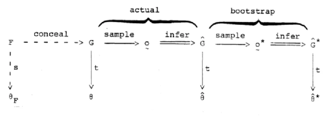
For instance, let’s consider F as a population of units 𝑌𝑡, where 𝑡 = 1,2, … , 𝑇, with T considered a big value. A missing data process, defined 𝑂𝑡 results in a population G of partially observed values. If the value of a parameter 𝜃𝐹 of the population F has to be inferred, a random sample
could be missing too. The empirical distribution 𝐺̂ of o is then used to estimate 𝜃𝐹, thanks to 𝜃̂ = 𝑡(𝐺̂) (Efron, 1994). From this point on, the bootstrapping procedure repeats the actual sampling, inference and estimation steps beginning with 𝐺̂ which, unlike G is known. Unlimited number of bootstrap replications can be done and each of them involves drawing a bootstrap sample 𝑜∗ from 𝐺̂ building the empirical distribution corresponding to the 𝑜∗ and
calculating 𝜃∗ = 𝑡(𝐺̂). ∗
The Figure 3 below, extracted from Efron (1994), shows in detail the process being descripted. The missing data problem does not affect directly F, rather than G. But, applying the bootstrap on these data, the missingness can be easily handled thanks to the number of inferences that can be done about the population through the sample-resample procedure.
Figure 3: Bootstrap procedure in a concealment process
Bootstrapping techniques can be used also if, instead of only estimating the parameters of a distribution, the missing values themselves have to be filled in. So, bootstrapping could also be one of the steps of an imputation technique. Indeed, if considering a variable 𝑌𝑡 𝑐𝑜𝑚, such that
𝑌𝑡 𝑐𝑜𝑚 = (𝑌𝑡 𝑜𝑏𝑠, 𝑌𝑡 𝑚𝑖𝑠), for each of the m imputed variables 𝑦𝑡 𝑚, n bootstrap samples are
drawn. Therefore, for each of the m x n datasets, the standard error of 𝜃̂𝑚, i.e. the parameter being estimated from each imputed variable, can be easily computed (Schomaker and Heumann, 2016; Shao and Sitter, 1996). In this case, the bootstrap is used to assess the goodness of the process of multiple imputation.
2.4.4
EMB
A
LGORITHMIn this paragraph, an algorithm developed by Honaker and King (2010) is described. This method combines, in order to take the best of all techniques, the Expectation-Maximization approach and the Bootstrap, in the context of the Multiple Imputation. This method was also built in order to take into account the trends in time and the shifts in space that a Time Series Cross Section (TSCS) dataset presents, which represents an advantage to this method. The idea of this algorithm arose from the computational difficulty in taking random draws of the
parameters of the variable from its posterior density, in order to represent the estimation uncertainty of the problem caused by the multiple imputations. The difficulty derives from the huge number of draws of parameters to be taken if considering a TSCS database. This step of the procedure is therefore replaced by a bootstrapping algorithm, a much faster application. Moreover, the other algorithms previously used to this aim like the Imputation-Posterior (IP) Approach and the Expectation Maximization importance sampling (EMis) require hundreds of lines of computer code to implement, while bootstrapping can be implemented in just a few lines. Furthermore, the variance matrix of the parameters does not need to be estimated, importance sampling does not need to be conducted and evaluated as in EMis (King et al., 2001) and Markov chains do not need to be burnt in and checked for convergence as in IP.
In detail, the so-called EMB algorithm starts drawing m samples of size n with replacement from the data yt, being m the number of imputations that will be done in the multiple imputation
part of the process. This first step is done through the bootstrapping technique. After obtaining these samples, the Expectation-Maximization algorithm produces reliable point estimates of the set of parameters being considered. Finally, for each set of estimates, the original sample unit is used to impute the missing data through the estimated parameters, keeping the original observed values (Honaker and King, 2010). The final result is a set of m multiply imputed datasets that can be combined following Rubin’s (1987) original rules, as already explained in the paragraph about the Multiple Imputation.
As explained by Efron (1994), the bootstrapped estimates of the parameters can be used in place of the draws from the posterior density because they have the right properties. Moreover, bootstrapping has lower order asymptotics than both IP and EMis approaches.
The EMB algorithm is a powerful technique because it combines the reliability of the Bootstrap together with the EM approach and the completeness of the Multiple Imputation. However, since it is thought to work with TSCS data, in order to apply it to a univariate time series, some adjustments in the software package Amelia II, i.e. the R-package created by Honaker and King (2010) to implement the EMB algorithm, have to be done. The procedure gives good and reliable results, especially if compared to those coming from the application of the single techniques being combined in the EMB algorithm.
2.4.5
M
ETHODS THAT DEAL WITHMNAR
DATAWhen the MCAR and the MAR assumptions do not hold, so the mechanism of missingness has to be included in the model being used to handle the dataset, the most part of the previous