Abstract
A novel numerical-experimental technique is developed in order to minimise some of the difficulties exhibited by others damage localisation approaches. The present technique relies on the computation of undamaged rotation fields using the Ritz method and the Timoshenko beam theory, while the measurement of damaged rotation fields is performed by speckle shear interferometry. Two damage localisation indicators are also presented, which, instead of being based on the second derivative of displacement fields, are based on the first spatial derivative of rotation fields. These damage localisation indicators, the modified curvature difference (MCD) and the modified damage index (MDI), were applied successfully in the localisation of damage in two clamped-clamped aluminium beams.
Keywords: damage detection, Ritz method, Timoshenko beam theory, rotation field, spatial derivative, shear interferometry.
1 Introduction
Structural damage identification methods have attracted the interest of mechanical, civil and aerospace engineering communities for the past decades. This interest is attested by the extensive number of papers, reviews and conferences dedicated to this area [1]. The underlying idea amongst most of these methods is that whenever there is damage in a structure, its stiffness, mass and damping properties change, therefore changing its dynamic behaviour.
Pandey et al. [2] developed the mode shape curvature, which allows the localisation of damage, since the curvatures are local properties, contrary to, for instance, natural frequencies. In their work the curvatures are computed by differentiating the displacement field using second order central finite differences. However, this numerical differentiation can lead to false localisations of damage, in
Paper
54
Damage Localisation in Beams using the
Ritz Method and Speckle Shear Interferometry
J.V. Araújo dos Santos
1, H.M.R. Lopes
2, J. Ribeiro
2N.M.M. Maia
1and M.A. Pires Vaz
31
IDMEC/IST, Instituto Superior Técnico, Lisboa, Portugal
2
ESTIG, Instituto Politécnico de Bragança, Portugal
3
DEMEGI, Faculdade de Engenharia do Porto, Portugal
©Civil-Comp Press, 2010
particular with sparse and noisy displacement fields. Indeed, with few measured points, the intrinsic error of the finite difference technique originates curvatures that can be far from the real ones. On the other hand, if the measurements are contaminated with noise, this noise is amplified by the differentiation. Instead of applying the second order central difference, Guan and Karbhari [3] proposed the use of a fourth order central difference method, therefore improving the results for sparse fields.
Stubbs
[4]presented t
he damage index method formulation which is based on mode shapes curvatures information. This damage index relates the second spatial derivative of the undamaged and damaged displacement fields in each segment or element of the structure. Over the years, several researchers have improved and applied curvature based methods to damage localisation in beam-like structures [5-16]. Usually, in these works, the curvatures are computed through the differentiation of relatively sparse displacement fields, and the damage indicators generally describe the state of damage in areas of the structures, i.e. the damage localization is performed element-by-element or segment-by-segment. Also, in most of these works, the beams were described assuming the Euler-Bernoulli assumptions, therefore limiting the applicability to thin beams.This paper is a contribution to minimise three of the main problems that mode shape curvature based methods present: (1) ineffective differentiation schemes, (2) lower spatial resolution, and (3) presence of noise in measurements. The first contribution is related to the first two problems. By using the Ritz method and the Timoshenko theory, one is able to compute the undamaged rotation field as a function series, and, therefore, the differentiation can be performed analytically. The damaged rotation field is obtained experimentally by speckle shear interferometry, which is a full-field technique, and the differentiation is performed through an efficient Gaussian function derivative. By combining both techniques, i.e. the Ritz method with the speckle shear interferometry, a point-by-point correlation of rotation fields and their spatial derivatives can be performed. The last problem, i.e.
the present of noise in the measurements, is coped by applying filters to the experimental data.
Two new damage localisation indicators are also presented in this paper. They are inspired on the mode shape curvature method, developed by Pandey et al. [2], and the damage index, proposed by Stubbs et al. [4]. However, instead of using the second spatial derivative of displacement fields, these novel indicators rely on the first spatial derivative of rotation fields. These indicators are applied to several cases of saw-cut damage in two aluminium beams. It is shown that most damages are successfully located and that both indicators values increase as the damage increases.
2 Methodology
2.1 Ritz method and Timoshenko beam theory
0
0 0
2
0 ⎟⎟ =
⎠ ⎞ ⎜⎜ ⎝ ⎛ − − ∂ ∂ ∂ ∂ + ∂ ∂ ∂ ∂
∫ ∫
T Ldt dx Q M t t m t w t w
m δ φ δ φ δκ δγ (1)
where m0 =ρA and m2 =ρAh2/12, being ρ the density, A the area, and h the beam thickness. Since ⎟⎟ ⎠ ⎞ ⎜⎜ ⎝ ⎛ + ∂ ∂ = ⎟⎟ ⎠ ⎞ ⎜⎜ ⎝ ⎛ ∂ ∂
=δ φ δγ δ φ
κ δ
x w
x , (2)
and the constitutive relations are
⎟⎟ ⎠ ⎞ ⎜⎜ ⎝ ⎛ + ∂ ∂ = ∂ ∂
= φ φ
x w GAK Q x EI
M , s (3)
where M is the bending moment, Q is the transverse (shear) force, E is the Young’s modulus, I is the second moment of area, Ks is the shear correction factor, and G is
the shear modulus, equation (1) can be written in terms of the displacement and rotation fieldsw(x,t), and φ(x,t), respectively:
0 0 0 2 0 = ⎥ ⎦ ⎤ ⎟⎟ ⎠ ⎞ ⎜⎜ ⎝ ⎛ + ∂ ∂ ⎟⎟ ⎠ ⎞ ⎜⎜ ⎝ ⎛ + ∂ ∂ − ∂ ∂ ∂ ∂ − ⎢ ⎣ ⎡ ∂ ∂ ∂ ∂ + ∂ ∂ ∂ ∂
∫ ∫
dt dx x w x w GAK x x EI t t m t w t w m s T L φ δ δ φ φ δ φ φ δ φ δ (4)Note that the first constitutive relation in Equation (3) shows that the flexural rigidity EI is associated, not with the second derivative of the displacement field
2 2
/ x
w ∂
∂ , as in a Euler-Bernoulli beam, but with the first spatial derivative of the rotation field ∂φ/∂x.
In the Ritz method for free vibration of a Timoshenko beam one seeks a 2N
parameter periodic analytical approximate solution of the form
∑
= = N j t i j jw x eW t x w 1 ) ( ) ,
( ω (5)
∑
= Φ = N j t i j j x et x 1 ) ( ) ,
( φ ω
φ (6)
mode shape described by the displacement field w(x,t) and the rotation field )
, (x t
φ . As can be seen, and contrary to the Euler-Bernoulli beam theory, in the present case we obtain directly the rotation field (Equation (6)), with no need to differentiate the displacement field (Equation (5)).
Substituting Equations (5) and (6) into Equation (4) results in an eigenvalue problem of order 2N:
KQ−ΛMQ=0 (7)
where Q and Λ contain the eigenvectors and the eigenvalues, respectively. Matrices K and M are partitioned by grouping the terms wi(x)wj(x), )wi(x)φj(x ,
) ( ) (x j x
i φ
φ and their partial derivatives, such that
( )
∫
∂ ∂ ∂ ∂
= L i j
s ij dx x x w x x w GAK 0 11 ) ( ) (
K (8)
( )
∫
∂ ∂ = L j i sij x dx
x x w GAK
0
12 ( )
)
( φ
K (9)
( )
∫
⎥ ⎦ ⎤ ⎢ ⎣ ⎡ + ∂ ∂ ∂ ∂ = L j i s j iij GAK x x dx
x x x x EI 0
22 ( ) ( )
) ( )
( φ φ φ
φ
K (10)
( )
( ) ( ) 00 0
11 =
∫
=L
j i
ij m w x w x dx
M (11)
(
)
( ) ( ) 00 2
22 =
∫
=L
j i
ij mφ x φ x dx
M (12)
In this work, the assumed functions wj(x) for the six different boundary conditions are the characteristic polynomials and are listed below [17].
• Simply supported - Simply supported (S-S): ) sin( )
(x x
wi = λi (13)
0 ) sin(
with λiL = (14)
• Clamped - Clamped (C-C):
[
cosh( ) cos( )]
) sinh( )
sin( )
(x x x x x
wi = λi − λi +αi λi − λi (15)
) cos( ) cosh( ) sin( ) sinh( and 0 1 ) cosh( ) ( cos with L L L L L L i i i i i i
i λ λ
λ λ α λ λ − − = =
• Clamped - Free (C-F):
[
cosh( ) cos( )]
) sinh( )
sin( )
(x x x x x
wi = λi − λi +αi λi − λi (17)
) cos( ) cosh( ) sin( ) sinh( and 0 1 ) cosh( ) ( cos with L L L L L L i i i i i i
i λ λ
λ λ α λ λ + + = =
+ (18)
• Simply supported - Clamped (S-C):
) sinh( ) sin( ) sin( ) sinh( )
(x L x L x
wi = λi λi − λi λi (19)
0 ) tanh( )
(
with tan λiL − λiL = (20)
• Simply supported - Free (S-F):
) sinh( ) sin( ) sin( ) sinh( )
(x L x L x
wi = λi λi + λi λi (21)
0 ) tanh( )
(
with tan λiL − λiL = (22)
• Free - Free (F-F):
[
cosh( ) cos( )]
) sinh( )
sin( )
(x x x x x
wi = λi + λi −αi λi + λi (23)
) cos( ) cosh( ) sin( ) sinh( and 0 1 ) cosh( ) ( cos with L L L L L L i i i i i i
i λ λ
λ λ α λ λ − − = =
− (24)
For most boundary conditions the roots λi of the characteristic equation must be computed using, for instance, the Newton-Raphson method. Since the present work relies on the Timoshenko beam theory, a set of assumed functions for the rotation field is also necessary. An appropriate set is given by
dx x dw x j j ) ( ) ( =
φ (25)
so that for beams with high length to thickness ratios the Euler-Bernoulli solution is recovered. This set of assumed functions also respects the boundary conditions relative to the mode shape slope.
2.2 Spatial derivatives of displacement and rotation fields
In this work we make use of higher order derivatives of displacement and rotation fields. Attending to Equations (5) and (6), the displacement and rotation fields n-th order spatial derivatives of the undamaged beam are given, respectively, by
∑
= = ∂ ∂ N j t i n j n j n n e dx x w d W x t x w 1 ) ( ) , ( ω (26)∑
= Φ = ∂ ∂ N j t i n j n j n n e dx x d x t x 1 ) ( ) ,( φ ω
φ
It should be noted that since the undamaged structure fields are described by an analytical expression, the differentiation does not involve any kind of numerical technique. This is not the case if these fields were, for instance, obtained by the finite element method.
The damage beam rotation field n-th order spatial derivatives are obtained through the one-dimensional n-th order Gaussian derivative:
) ( 2 2
1 )
(
x G x H x
d x G d
n n
n
⎟ ⎠ ⎞ ⎜ ⎝ ⎛ ⎟ ⎠ ⎞ ⎜ ⎝ ⎛ =
π
π (28)
where
⎟⎟ ⎠ ⎞ ⎜⎜ ⎝ ⎛ − =
2 exp 2 1 ) (
2
x x
G
π (29)
and )Hn(x are the Hermite polynomials:
) ( ) 1 ( 2 ) ( 2 ) (
2 ) (
1 ) (
1 1
1 0
x H n x xH x
H
x x H
x H
n n
n+ = − − −
= =
(30)
This differentiation scheme has also the capability to smooth the measured data, therefore decreasing the influence of noise. A comprehensive description of this technique can be found in references [18-19].
2.3 Shear
interferometry
The digital shearography technique is a powerful tool that allows non-contact and full-field measurements of surface out-of-plane spatial gradients of displacement fields. The shear interferometer technique proposed by [18-19] granted the direct measurement of modal rotation fields in a free-free plate excited acoustically at its natural frequencies by using a loudspeaker. In this set-up a spatial carrier is introduced in the hologram primary fringes in order to perform the phase map calculation [20]. However, it produces high levels of speckle noise in the measurements. The use of image processing techniques allows the elimination of this speckle noise, but the perturbations due to damage in the modal response fields are also eliminated in this process. This is one of the reasons why this technique presents some difficulties in localising damage.
laser using an acousto-optic modulator [22]. Any point of the beam vibration cycle is illuminated with short stroboscopic pulses synchronized with its vibration excitation. The beam modal rotation fields are obtained by filtering and unwrapping the measurement phase maps. Afterwards, these fields are post-processed in order to obtain the modal rotation spatial derivatives. Dedicated image processing algorithms proposed by [18-19] were used in this process.
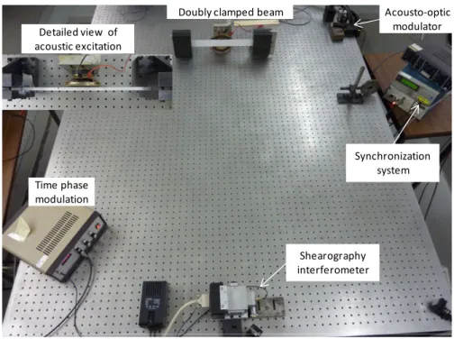
The measurements used in this work were performed in two aluminium beams. The beams were fixed at both ends by using two rigid blocks. A general view of the experimental set-up, used for modal rotation field measurement on the beam with different damages severities are shown in Figure 1.
Shearography interferometer Detailed view of
acoustic excitation
Doubly clamped beam
Time phase modulation
Acousto‐optic modulator
Synchronization system
Figure 1: General view of experimental set-up for the measurement of rotation fields.
3 Preliminary analysis
This section presents a preliminary analysis of the rotation fields and their spatial derivatives of an undamaged beam obtained using the Ritz method. The objective is to show that, for relatively thick beams, the spatial derivative of the displacement field is not equal to the rotation field, and the same applies for higher derivatives. In order to do that, beams with 1 m x 0.25 m, E = 210 GPa, ν = 0.3, ρ= 7800 kg/m3,
Ks = 5/6, and different thicknesses and boundary conditions were studied.
The spatial derivatives were compared by computing the relative difference between a vector φ(k) and a vector w(k+1), whose entries are, respectively,
k l
k
x t
x ∂
∂ φ( , )/ and ∂(k+1)w(xl,t)/∂x(k+1), for xl =0,…,L with an increment of
NP
2 ) (
2 ) 1 ( ) (
k k k
φ
w
φ − +
(31)
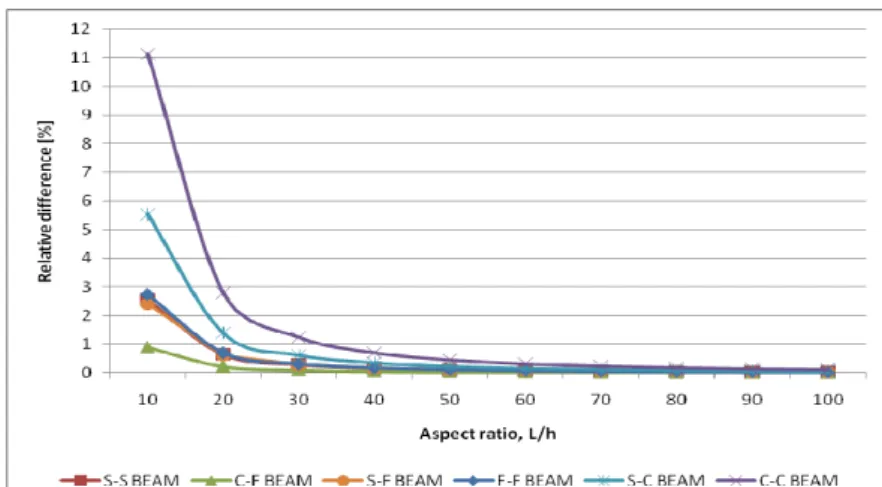
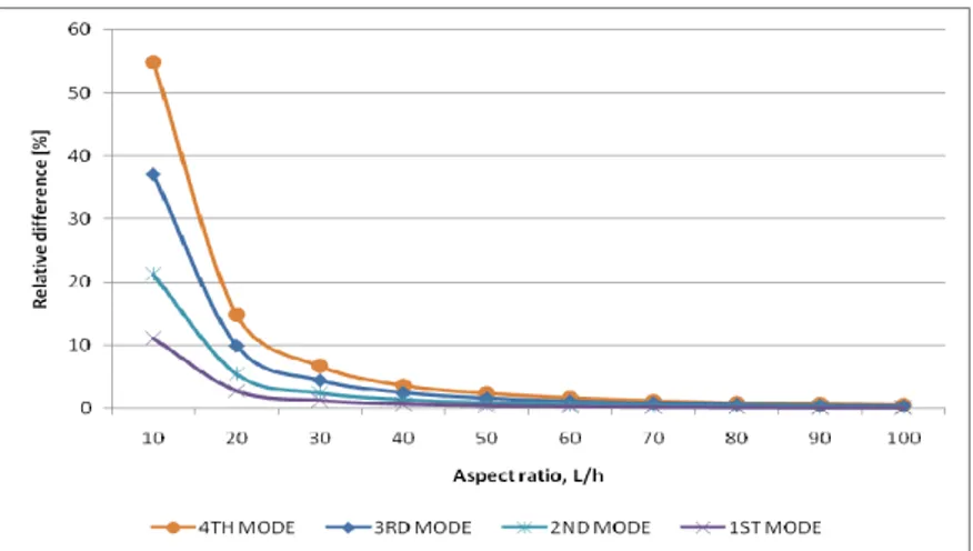
Figure 2 shows the relative differences between rotation fields and displacement fields first derivative for beams with different boundary conditions and aspects ratios of the first mode. As expected, for relatively high aspect ratios the differences are minimal. One sees that the C-C beam is the beam presenting the greatest differences, while the C-F beams has the minor differences. This trend is also observed in differences of higher order derivatives of w and φ, such as those between ∂2φ/∂x2and ∂3w/∂x3, and between ∂3φ/∂x3 and ∂4w/∂x4. Note that the comparative results here presented, for vectors with length NP=101, do not depend on the size of φ(k) and w(k+1).
Figure 2: Relative differences between φ(x)and ∂w/∂x of the first mode as function of aspect ratio L/h for different boundary conditions.
Figure 3: Relative differences between φ(x)and ∂w/∂x of a C-C beam as function of aspect ratio L/h and mode shape.
4 Damage localisation
Two aluminium clamped-clamped beams with 351 mm x 40 mm were studied in this work. The beams are 2.1 mm and 8 mm thick. Both beams were subjected to several cases of damaged characterised by performing a cut trough the beams width at coordinate x = 90 mm (Figure 4). Table 1 presents the depths of the cuts performed. All the cuts are 1 mm length (c = 1 mm).
Figure 4: Damage dimensions
Damage Depth, p (Beam 1) Depth, p (Beam 2)
case (mm) (mm) 1 0.3 0.8 2 0.5 1.2 3 1.0 1.6
4 — 2.0
5 — 4.0
Table 1: Damage dimensions
dx x d dx x d x
i i l i l
l ) ( ) ( ~ ) , (
MCD = φ − φ (32)
∑
∑
∑
∑
= = = = ⎟⎟ ⎠ ⎞ ⎜⎜ ⎝ ⎛ ⎥ ⎥ ⎦ ⎤ ⎢ ⎢ ⎣ ⎡ ⎟ ⎠ ⎞ ⎜ ⎝ ⎛ + ⎟ ⎠ ⎞ ⎜ ⎝ ⎛ ⎟ ⎠ ⎞ ⎜ ⎝ ⎛ ⎥ ⎥ ⎦ ⎤ ⎢ ⎢ ⎣ ⎡ ⎟⎟ ⎠ ⎞ ⎜⎜ ⎝ ⎛ + ⎟⎟ ⎠ ⎞ ⎜⎜ ⎝ ⎛ = NP k k i NP k k i l i NP k k i NP k k i l i l dx x d dx x d dx x d dx x d dx x d dx x d x i 1 2 1 2 2 1 2 1 2 2 ) ( ~ ) ( ) ( ) ( ) ( ~ ) ( ~ ) , ( MDI φ φ φ φ φ φ (33)where i denotes the mode shape, xl is the coordinate where the first spatial derivative of the maximum amplitudes of the undamaged and damaged of rotation fields )φ(x,t and )φ~(x,t , respectively, are computed and NP is the number of measured points. Since both beams have the same in-plane dimensions, the number of measured points is also the same and equal to 2158. This high number of measured points is only possible because we are using shear interferometry to measure the experimental damaged rotation field and analytically computing the equivalent undamaged field. Recall that most works on damage localisation reported in the literature rely on techniques that use accelerometers or laser vibrometers. In general, these techniques only allow the measurement of sparse displacement fields and are very time consuming. Also, the undamaged rotation fields are usually obtained using finite elements, which implies that their derivatives must be computed using some kind of numerical differentiation scheme. The standard mode shape curvatures differences (e.g. [2]) and damage index (e.g. [4]) are recovered if we consider the Euler-Bernoulli assumptionφ(x)=dw/dx. In other words, the standard damage indicators are function of the second derivative of the displacement field, not the first derivative of the rotation field.
4.1 Beam
1
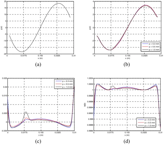
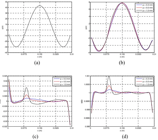
Figures 5(a) and (b) show the first mode rotation fields of Beam 1 in the undamaged and damaged states, respectively. Although the values have different magnitudes we see that the undamaged and damaged shapes are similar and that only for a high damage slight perturbations are observed in the damaged rotation field. These perturbations are not necessarily located at the damage position.
0 0.0775 0.155 0.2325 0.31 -20
-15 -10 -5 0 5 10 15 20
x (m)
φ
(x
)
0 0.0775 0.155 0.2325 0.31
-4 -3 -2 -1 0 1 2 3 4
x (m)
φ
(x
)
p = 0.3 mm p = 0.5 mm p = 1.0 mm
(a) (b)
0 0.0775 0.155 0.2325 0.31
-0.005 0 0.005 0.01 0.015 0.02 0.025
x (m)
MC
D
p = 0.3 mm p = 0.5 mm p = 1.0 mm
0 0.0775 0.155 0.2325 0.31
0.9986 0.9988 0.999 0.9992 0.9994 0.9996 0.9998 1 1.0002 1.0004
x (m)
MD
I
p = 0.3 mm p = 0.5 mm p = 1.0 mm
(c) (d)
Figure 5: First mode (a) undamaged rotation field, (b) damaged rotation fields, (c) MCD, and (d) MDI of Beam 1
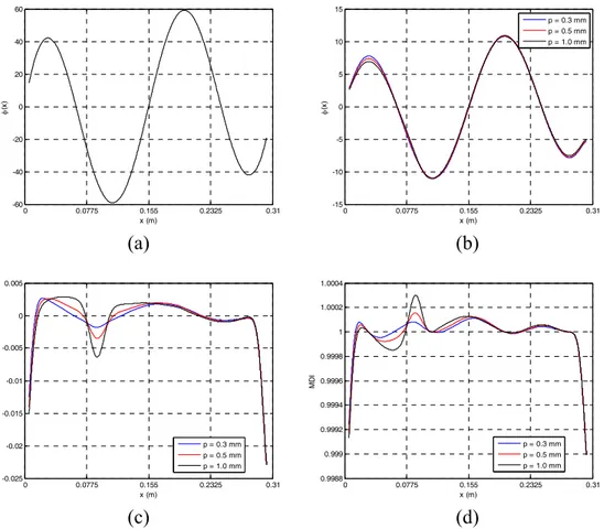
The first mode MCD and MDI are presented in Figures 5(c) and (d), respectively. We see that near the borders the MCD and MDI present maximum or minimum values. This is also observed in the second and third modes (Figures 6 and 7) thus indicating that this is a systematic behaviour and can not be justified by the presence of damage. This is due, among other factors, to difficulties in accomplishing a perfect clamping of the beam and errors in the computation of the experimental derivatives of the rotation fields [19]. There is another systematic presence of stationary points of both damage indicators at coordinates where φ(x)=0. This is particularly clear in the third mode and MDI (Figures 7(d)). Therefore, one can conclude that lower modes yield better damage localisations than higher modes, since these stationary points may be mistaken for damage locations. At a coordinate
09 . 0
≈
0 0.0775 0.155 0.2325 0.31 -40
-30 -20 -10 0 10 20 30 40 50
x (m)
φ
(x
)
0 0.0775 0.155 0.2325 0.31
-6 -4 -2 0 2 4 6 8
x (m)
φ
(x
)
p = 0.3 mm p = 0.5 mm p = 1.0 mm
(a) (b)
0 0.0775 0.155 0.2325 0.31
-0.025 -0.02 -0.015 -0.01 -0.005 0 0.005 0.01 0.015 0.02 0.025
x (m)
MC
D
p = 0.3 mm p = 0.5 mm p = 1.0 mm
0 0.0775 0.155 0.2325 0.31
0.998 0.9985 0.999 0.9995 1 1.0005 1.001
x (m)
MD
I
p = 0.3 mm p = 0.5 mm p = 1.0 mm
(c) (d)
Figure 6: Second mode (a) undamaged rotation field, (b) damaged rotation fields, (c) MCD, and (d) MDI of Beam 1
4.2 Beam
2
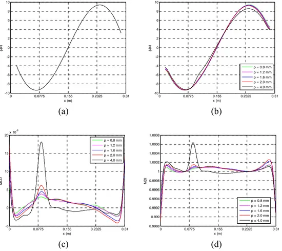
To verify the appropriateness and reproducibility of the proposed approach a second beam was studied. The first mode alone was considered and its undamaged and damaged rotation fields are shown in Figure 8(a) and (b). Like was found in Beam 1, we see that most damaged shapes are similar to the undamaged one. Only the larger damage presents a rotation field with a noticeable perturbation between coordinates
0775 . 0
=
0 0.0775 0.155 0.2325 0.31 -60
-40 -20 0 20 40 60
x (m)
φ
(x
)
0 0.0775 0.155 0.2325 0.31
-15 -10 -5 0 5 10 15
x (m)
φ
(x
)
p = 0.3 mm p = 0.5 mm p = 1.0 mm
(a) (b)
0 0.0775 0.155 0.2325 0.31
-0.025 -0.02 -0.015 -0.01 -0.005 0 0.005
x (m)
MC
D
p = 0.3 mm p = 0.5 mm p = 1.0 mm
0 0.0775 0.155 0.2325 0.31
0.9988 0.999 0.9992 0.9994 0.9996 0.9998 1 1.0002 1.0004
x (m)
MD
I
p = 0.3 mm p = 0.5 mm p = 1.0 mm
(c) (d)
Figure 7: Third mode (a) undamaged rotation field, (b) damaged rotation fields, (c) MCD, and (d) MDI of Beam 1
5 Conclusions
0 0.0775 0.155 0.2325 0.31 -10
-8 -6 -4 -2 0 2 4 6 8 10
x (m)
φ
(x
)
0 0.0775 0.155 0.2325 0.31
-10 -8 -6 -4 -2 0 2 4 6 8 10
x (m)
φ
(x
)
p = 0.8 mm p = 1.2 mm p = 1.6 mm p = 2.0 mm p = 4.0 mm
(a) (b)
0 0.0775 0.155 0.2325 0.31
-5 0 5 10 15 20x 10
-3
x (m)
MC
D
p = 0.8 mm p = 1.2 mm p = 1.6 mm p = 2.0 mm p = 4.0 mm
0 0.0775 0.155 0.2325 0.31
0.9988 0.999 0.9992 0.9994 0.9996 0.9998 1 1.0002 1.0004 1.0006 1.0008
x (m)
MD
I
p = 0.8 mm p = 1.2 mm p = 1.6 mm p = 2.0 mm p = 4.0 mm
(c) (d)
Figure 8: First mode (a) undamaged rotation field, (b) damaged rotation fields, (c) MCD, and (d) MDI of Beam 2
Acknowledgements
The authors greatly appreciate the financial support of FCT through Project FCT PTDC/EME-PME/102095/2008.
References
[1] J.V. Araújo dos Santos, N.M.M. Maia, C.M. Mota Soares, C.A. Mota Soares, “Structural Damage Identification: A Survey”, in B.H.V. Topping, M. Papadrakakis, (Editors), “Trends in Computational Structures Technology”, Saxe-Coburg Publications, Stirlingshire, UK, Chapter 1, 1–24, 2008.
[2] A.K. Pandey, M. Biswas, M.M. Samman, “Damage Detection from Changes in Curvature Mode Shapes”, Journal of Sound and Vibration, 145(2), 321– 332, 1991.
[4] N. Stubbs, J.T. Kim, C.R. Farrar, “Field Verification of a Nondestructive Damage Localization and Severity Estimation Algorithm”, in “Proceedings of the 13th International Modal Analysis Conference”, Nashville, U.S.A., 210– 218, 1995.
[5] O.S. Salawu, C. Williams, “Damage Location Using Vibration Mode Shapes”, in “Proceedings of the 12th International Modal Analysis Conference”, Honolulu, Hawai, U.S.A., 933–939, 1994.
[6] N. Stubbs, J.T. Kim, “Damage Localization in Structures Without Baseline Modal Parameters”, AIAA Journal, 34, 1644–1649, 1996.
[7] J.T. Kim, N. Stubbs, “Crack Detection in Beam-Type Structures Using Frequency Data”, Journal of Sound and Vibration, 259, 145–160, 2003.
[8] C.P. Ratcliffe, W.J. Bagaria, “Vibration Technique for Locating Delamination in a Composite Beam”, AIAA Journal, 36, 1074–1077, 1998.
[9] J. Maeck, G. De Roeck, “Dynamic Bending and Torsion Stiffness Derivation from Modal Curvatures and Torsion Rates”, Journal of Sound and Vibration, 225, 153–170, 1999.
[10] N.M.M. Maia, J.M.M. Silva, R.P.C. Sampaio, “Localization of Damage Using Curvature of the Frequency-Response-Functions”, in “Proceedings of the 15th International Modal Analysis Conference”, Orlando, Florida, USA, 942–946, 1997.
[11] R.P.C. Sampaio, N.M.M. Maia, J.M.M. Silva, “Damage Detection Using the Frequency-Response-Function Curvature Method”, Journal of Sound and Vibration, 226, 1029–1042, 1999.
[12] A. Dutta, S. Talukdar, “Damage Detection in Bridges Using Accurate Modal Parameters”, Finite Elements in Analysis and Design, 40, 287–304, 2004. [13] C.S. Hamey, W. Lestari, P. Qiao, G. Song, “Experimental Damage
Identification of Carbon/Epoxy Composite Beams Using Curvature Mode Shapes”, Structural Health Monitoring, 3, 333–353, 2004.
[14] W. Lestari, P. Qiao, “Damage Detection of Fiber-Reinforced Polymer Honeycomb Sandwich Beams”, Composite Structures, 67, 365–373, 2005. [15] W. Lestari, P. Qiao, S. Hanagud, “Curvature Mode Shape-based Damage
Assessment of Carbon/Epoxy Composite Beams”, Journal of Intelligent Material Systems and Structures, 18, 189–208, 2007.
[16] M. Chandrashekhar, R. Ganguli, “Damage assessment of structures with uncertainty by using mode-shape curvatures and fuzzy logic”, Journal of Sound and Vibration, 326 (3-5), 939-957, 2009.
[17] J.N. Reddy, “Energy Principles and Variational Methods in Applied Mechanics”, John Wiley and Sons, Hoboken, New Jersey, 2nd edition, 2002. [18] J.V. Araujo dos Santos, H.M.R. Lopes, M. Vaz, C.M. Mota Soares, C.A. Mota
Soares, M.J.M. de Freitas, “Damage localization in laminated composite plates using mode shapes measured by pulsed TV holography”, Composite Structures, 76, 272–281, 2006.
[20] G. Pedrini, B. Pfister, H. Tiziani, “Double Pulse-Electronic Speckle Interferometry”, Journal of Modern Optics, 40, 89–96, 1993.
[21] T. Kreis, “Handbook of Holographic Interferometry: Optical and Digital Methods”, WILEY-VCH GmbH & Co. KGaA, 2005.