ISSN 1549-3636
© 2005 Science Publications
Corresponding Author : Luai Al Shalabi, Faculty of Computer Science and Information Technology, Applied Science University, Jordan
Data Mining: A Preprocessing Engine
Luai Al Shalabi, Zyad Shaaban and Basel Kasasbeh
Applied Science University, Amman, Jordan
Abstract: This study is emphasized on different types of normalization. Each of which was tested against the ID3 methodology using the HSV data set. Number of leaf nodes, accuracy and tree growing time are three factors that were taken into account. Comparisons between different learning methods were accomplished as they were applied to each normalization method. A new matrix was designed to check for the best normalization method based on the factors and their priorities. Recommendations were concluded.
Key words: Transformation, normalization, induction decision tree, rules generation, KNN, LTF_C
INTRODUCTION
Induction decision tree (ID3)[1] algorithm implements a scheme for top-down induction of decision trees using depth-first search. The input to the algorithm is a tabular set of training objects, each characterized by a fixed number of attributes and a class designation. ID3 is one of the most common techniques used in the field of data mining and knowledge discovery.
Data usually collected from multiple resources and stored in data warehouse. Resources may include multiple databases, data cubes, or flat files. Different issues could arise during integration of data that we wish to have for mining and discovery. These issues include scheme integration and redundancy. So, data integration must be done carefully to avoid redundancy and inconsistency that in turn improve the accuracy and speed up the mining process[2].
The careful data integration is now acceptable but it needs to be transformed into forms suitable for mining. Data transformation involves smoothing, generalization of the data, attribute construction and normalization.
Data mining seeks to discover unrecognized associations between data items in an existing database. It is the process of extracting valid, previously unseen or unknown, comprehensible information from large databases. The growth of the size of data and number of existing databases exceeds the ability of humans to analyze this data, which creates both a need and an opportunity to extract knowledge from databases[3].
Data transformation such as normalization may improve the accuracy and efficiency of mining algorithms involving neural networks, nearest neighbor and clustering classifiers. Such methods provide better results if the data to be analyzed have been normalized, that is, scaled to specific ranges such as [0.0, 1.0][2].
An attribute is normalized by scaling its values so that they fall within a small-specified range, such as 0.0 to 1.0. Normalization is particularly useful for classification algorithms involving neural networks, or distance measurements such as nearest neighbor classification and clustering. If using the neural network back propagation algorithm for classification mining, normalizing the input values for each attribute measured in the training samples will help speed up the learning phase. For distanced-based methods, normalization helps prevent attributes with initially large ranges from outweighing attributes with initially smaller ranges[2]. There are many methods for data normalization include min-max normalization, z-score normalization and normalization by decimal scaling.
Min-max normalization performs a linear transformation on the original data. Suppose that mina
and maxa are the minimum and the maximum values for
attribute A. Min-max normalization maps a value v of A to v’ in the range [new-mina, new-maxa] by
computing:
v’= ( (v-mina) / (maxa – mina) ) * (new-maxa –
new-mina) + new-mina
In z-score normalization, the values for and attribute A are normalized based on the mean and standard deviation of A. A value v of A is normalized to v’ by computing:
v’ = ( ( v – ) / A )
where and A are the mean and the standard
deviation respectively of attribute A. This method of normalization is useful when the actual minimum and maximum of attribute A are unknown.
Normalization by decimal scaling normalizes by moving the decimal point of values of attribute A. The number of decimal points moved depends on the maximum absolute value of A. A value v of A is normalized to v’ by computing:
where j is the smallest integer such that Max(|v’|)<1.
Normalization can change the original data and it is necessary to save the normalization parameters (the mean and the standard deviation if using the z-score normalization and the minimum and the maximum values if using the min-max normalization) so that future data can be normalized in the same manner.
METHODOLOGY
In this study, three different normalization methods were considered: z-score normalization, min-max normalization and decimal point normalization. HSV data set was used which consists of 122 examples. The data set has no missing values and it was taken from the UCI repository[4].
HSV data set was experimented in two ways. First, the entire HSV data set which consists of 122 examples was considered as a training set and no testing set was required. Secondly, the data set was fragmented into two subsets: the training set which consists of 75% of the original HSV data (92 examples) and the testing set which consists of the 25% of the original HSV data (30 examples). The reason behind using the training set of 122 examples and the training set of 92 examples is to check the effect of number of examples in the training set on the accuracy, the simplicity and the tree growing time. Al Shalabi has tested the HSV data against mini-max normalization method[5]. This study was extended to take into account z-score and decimal scaling normalization methods. Comparisons between the three normalization methods were discussed in this paper.
HSV data set was normalized using the three methods of normalization that were mentioned earlier. We used two training data sets for each normalization method: the training data set of 122 training examples (the original data set) and the training data set of 92 training examples (75% of original data set). T1, T2 and T3 are the training data sets of 122 training examples that are generated from min-max, z-score and decimal scaling normalization methods respectively. While T1’, T2’ and T3’ are the training data sets of 92 training examples that are generated from min-max, z-score and decimal scaling normalization methods respectively.
Decision tree methodology for data mining and knowledge discovery[4] was used to test the six training data sets that were designed earlier. For each data set, the accuracy, the simplicity and the tree growing time were computed.
K-Nearest Neighbor (KNN)[3,6], Local Transfer Function Classifiers (LTF-C) which is a classification-oriented artificial neural network model[7] and rule based classifier[4] are three methods used for data mining. The study is extended to test the accuracy by applying the above three data mining techniques to T1, T2 and T3 training data sets.
THE PREFERENCE MATRIX APPROACH
It is well known that different techniques usually generate different results when they are applied to a specific task. A data set can be redesigned in some way that helps techniques to generate better results. For
example, rules generation technique could give low accuracy when it is applied to decimal scaling normalization data set, while it gives much better accuracy when it is applied to z-score or min-max normalization data sets. Designing a task in some way could help in generating better accuracy.
A new approach is evaluated here. The new designed preference matrix is a simple way to choose the best normalization method between numbers of normalization methods that are used to test a specific data set.
High simplicity, high accuracy and low tree growing time are all preferred to be generated. A data set that is designed in different ways could get different results based on how the design is accomplished. If we choose the design that gives high simplicity, then we may get low accuracy or high tree growing time. Also, if we choose the data set design that gives the highest accuracy and simplicity, then this design could give us a very long tree growing time which is not preferred specially if the data set is dynamic.
The new preference matrix can help in choosing the best data set design that takes into account the best of each factor. It consists of columns that represent the preferred factors and rows that represent the different data set design. Numbers starting from 1…n represents each factor. Each number represents the priority that this factor is highly accepted for this data set design. For simplicity, the minimum number of leaf nodes is represented as 1. Two different data sets design could have the same priority if they have the same number of leaf nodes. It is the same for the tree growing time factor. The lowest tree growing time is represented as 1 (priority 1) and the highest priority is for the data set design that takes highest tree growing time. When accuracy factor is used, the highest accuracy is represented as 1. The next higher accuracy is represented as 2 and so on.
The last column of the preference matrix represents the summation of all priorities. Each row’s value in the last column represents the summation of all priorities in the same row. The minimum number in the last column of the matrix is considered the highest priority and then the designed data set of that row is the best data set design that we wish to achieve. We remember that this data set has the best design if we take into account all the three factors. If we are looking for higher accuracy regardless the simplicity or the tree growing time, another data set could be the best one to use.
This approach is also used when rows represent different data set designs and columns represent different data mining techniques that generate accuracy. The best data set design is the one where many techniques give high accuracy when they performed on it. The minimum number of summation of priorities for a specific data set is the best one. So, the data set that corresponds to that minimum summation has the best design.
RESULTS AND DISCUSSION
Table 1: Results of the three different approaches
Approach Min-max HSV Z-score HSV Decimal scaling HSV
Data Set T1 T1' T2 T2' T3 T3'
Accuracy 94.2 75.7 92 81.7 92 74.9
Tree growing time/sec 68 46 70 51 184 118
# of leaf nodes 27 19 26 20 26 17
Table 2: Priorities of the three different approaches when they are applied to HSV data sets of 122 and 92 training examples. Shaped pixels in the same column are of same priority
Data set size Original DS 75% of the original DS
Original DS 75% of the original DS
Original DS 75% of the
original DS Factors # of leaf nodes # of leaf nodes Accuracy Accuracy Tree growing time Tree growing time
Z-score Decimal point Min-max Z-score Min-max Min-max
Decimal point Min-max Z-score Min-max Z-score Z-score
higher priority
Min-max Z-score Decimal point Decimal point Decimal point Decimal point
Table 3: The accuracy of different data mining techniques
The technique Min-max accuracy (%) Z-score accuracy (%) Decimal point accuracy (%)
Rules generation 100 100 35.2
KNN 66.4 66.4 66.4
LTF_C 66.4 62.3 66.4
Table 4: Priorities of the three different data mining techniques as they are applied to HSV data sets of 122 training examples. Shaped pixels are of same priority
Accuracy Priorities Rule generation KNN LTF-C
Min-max Min-max Min-max
Z-score Z-score Decimal point
Higher priority
Decimal point Decimal point Z-score
Original DS # of leaf Accuracy Tree growing Summation
nodes time
Z-score 1 2 2 5
Min-max 2 1 1 4
Decimal point 1 2 3 6
Fig. 1: Matrix 1 which describes the evaluation against the entire data set of 122 training examples
75% of original DS # of leaf Accuracy Tree growing Summation
nodes time
Z-score 3 1 2 6
Min-max 2 2 1 5
Decimal point 1 3 3 7
Fig. 2: Matrix 2 which describes the evaluation against the training data set of 92 training examples
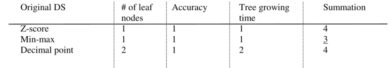
Original DS # of leaf Accuracy Tree growing Summation
nodes time
Z-score 1 1 1 4
Min-max 1 1 1 3
Decimal point 2 1 2 4
Fig. 3: Matrix 3 which describes the accuracy evaluation of the training data set of 122 training examples
The accuracy, the simplicity and the tree growing time are all reported for each normalization method.
Number of leaf nodes that represents the simplicity was generated for each training data set of 122 examples that were demonstrated by T1, T2 and T3. Number of leaf nodes is 27, 26 and 26 respectively. The
nods). The next higher simplicity was generated from the min-max normalization data set (19 leaf nodes). The z-score normalization data set generated the lowest simplicity as ID3 methodology built a tree of 20 leaf nodes.
When ID3 was applied to T1, T2 and T3, the accuracy results were as follows 94.2%, 92% and 92% respectively. The higher accuracy was noticed when the min-max normalization data set is used. The next higher accuracy was when the z-score and the decimal point normalization data sets were used. If T1’, T2’ and T3’ were considered, then the higher accuracy was when the z-score normalization data set was used (81.7%). The min-max normalization data set is in the second place as it gave accuracy of 75.7%. The lowest accuracy was 74.9% and it was generated from the decimal point normalization data set.
The tree growing time was computed for T1, T2 and T3 data sets and results were 68, 70 and 184 seconds respectively. The shortest training time was when the min-max normalization data set was trained and which took 68 seconds. ID3 took 70 seconds to train the z-score normalization data set in order to generate the tree. While it took 184 seconds to train the decimal point normalization data set. The training time of the decimal point data set was a very long time comparing to the other two times of training the min-max and the z-score normalization data sets. When ID3 trains T1’, T2’ and T3’ data sets, the same priorities of the tree growing time were achieved. Results were 46, 51 and 118 seconds respectively.
Table 2 summarizes the priorities of the normalization data sets based on the three factors (number of leaf nodes, accuracy and tree growing time) in both the data set of 122 training examples and the data set of 92 training examples.
The preference matrix is built to handle the three factors and the three normalized data sets. Results are summarized in Fig. 1 and 2. Matrix 1 is handling T1, T2 and T3 whereas matrix 2 is handling T1’, T2’ and T3’ As in the preference matrix 1, the best normalization data set was the min-max data set as it gave the minimum summation. For the min-max data set, the priorities of the simplicity, the accuracy and the tree growing time were 2, 1 and 1 respectively, which gave the summation value 4. The z-score normalization data set has 1, 2 and 2 priorities for the simplicity, the accuracy and the tree growing time respectively. The summation value of these priorities was 5. The decimal point normalization data set has priorities summarizes as 1, 2 and 3 for the simplicity, the accuracy and the tree growing time respectively and the summation of these priorities was 6. The next best normalization data set was the z-score data set as it gave the summation result 5. The worst normalization data set was the decimal scaling data set as it gave the highest summation value, which was 6.
When the preference matrix 2 is built to handle the three data sets of 92 training examples, the best normalization data set was the min-max data set. It gave the minimum summation value. The z-score normalization data set was the second choice whereas the decimal point normalization data set was in the last place.
New tests were performed to evaluate the preference matrix approach that takes into account the best of each data mining technique. Results that we get were described by the accuracy of different data mining techniques that were applied to each normalization data set. The experiment has performed on the normalized data set of 122 training examples. Table 3 summarizes the accuracy of different data mining techniques. The rules generation technique gave 100% accuracy when it was applied to the z-score and the min-max data sets. While it gave low accuracy when it was applied to the decimal point data set (35.2%). The KNN technique gave the same accuracy when it was applied to all the three normalization data sets and the accuracy was 66.4%.
Finally, the LTF_C was applied. It gave the same accuracy as it is applied to the min-max and the decimal point normalization data sets that was 66.4%. The accuracy was 62.3% when the same technique was applied to the z-score normalization data set.
Table 4 describes the priorities of the three techniques (as factors) when they were applied to the specific normalization data sets. Preference matrix 3 shows the summation of priorities of each factor (the data mining techniques). The min-max normalization data set has the summation value 3, the z-score normalization data set has the summation value 4 and the decimal scaling normalization data set has the summation value 4. It means that the best normalization data set that different techniques prefer is the min-max normalization because it has the minimum summation value. Next preference was either the z-score or the decimal scaling normalization data sets because they have the same summation values.
CONCLUSION
The experimental results suggested choosing the min-max normalization data set as the best design for training data set. In all experiments, the min-max normalization data set always has the highest priority because of the following reasons:
* The min-max normalization data set is always has the highest accuracy when the whole HSV data set is learned using the rule generation, KNN, LTF_C, or ID3 methodology.
* The min-max normalization data set has the least complexity when ID3 methodology is learning the whole HSV data set. ID3 generates the minimum number of nodes.
* The min-max normalization data set has the lowest tree growing time, so it is the faster than the other two methods of normalization.
* The new preference matrix is a suitable approach that helps in choosing the best normalization data set. It shown reasonable results as discussed earlier. * Preparing data that best support the classifier is all what we wish to achieve. The best-preprocessed data (normalized data) is best chosen by the use of the preference matrix that was proposed in this paper.
REFERENCES
1. Quinlan, J.R., 1986. Induction of Decision Trees. Machine Learning. Kluwer Academic Publishers, 1986 : 81-106.
2. Han, J. and M. Kamber, 2001. Data Mining: Concepts and Techniques, Morgan Kaufmann, USA.
3. Gora, G. and A. Wojna, (2002). RIONA: A new classification system combining rule induction and instance-based learning. Fundamenta Informaticae, 51: 369-390.
4. Mertz, C.J. and P.M. Murphy, 1996. UCI Repository of machine learning databases. http://www.ics.uci.edu/~mlearn/MLRepository.htm l”, University of California, 1996.
5. Al-Shalabi, L., 2006. Coding and normalization: The effect of accuracy, simplicity and training time. RCED’05, Al-Hussain Bin Talal University, Accepted.
6. Gora, G and A Wojna, 2002. RIONA: A classifier combining rule induction and k-NN method with automated selection of optimal neighbourhood. Proc. Thirteenth Eur. Conf. Machine Learning. ECML, Helsinki, Finland, Lecture Notes in Artificial Intelligence, 430. Springer-Verlag, pp: 111-123.