The annual cycle of satellite derived sea surface temperature on the western South Atlantic shelf

Rev. bras. oceanogr.. 48(2):93-105. 2000

The annual cycle of satellite derived sea surface temperature on the

western South Atlantic shelf

Carlos A. D. Lentini1; Edmo J. D. Campos2& Guillermo G. Podestá1

lRosenstiel School ofMarine and Atmospheric Science Division ofMeteorology and Physical Oceanography (4600 Rickenbacker Causeway, Miami, FL 33149-1098, USA)

Phone: (305) 361-4628 Fax: (305) 361-4696 E-mail: clentini@rsmas.miami.edu

2Instituto Oceanográfico da Universidade de São Paulo Departamento de Oceanografia Física

(Caixa Postal 66149, 05315-970 São Paulo, SP, Brasil)

.

Abstract: ln this article, thirteen years of weekly sea surface temperature (SST) fields derived trom NOAA Advanced Very High Resolution Radiometer global area coverage intrared sateIlite data, trom January 1982 to December 1994, are used to investigate spatial and temporal variabilities of SST seasonal cycle in the Southwest Atlantic Oceano This work addresses large scale variations over the eastern South American continental shelf and slope regions limited offshore by the 1000-m isobath, between 42° and 22°S. SST time series are fit with annual and semi-annual harmonics to describe the annual variation of sea surface temperatures. The annual harmonic explains a large proportion of the SST variability. The coefficient of determination is highest (> 90%) on the continental shelf, decreasing offshore. The estimated amplitude of the seasonal cycle ranges between 4° and 13°e throughout the study area, with minima in August-September and maxima in February-March. After the identification and removal of the dominant annual components of SST variability, models such as the one presented here are an attractive tool to study interannual SST variability.

.

Resumo: Neste artigo, treze anos de imagens semanais da temperatura da superficie do mar (TSM) obtidas através do sensor intravermelho Advanced Very High Resolution Radiometer a bordo dos satélites NOAA, de janeiro de 1982 a dezembro de 1994, são utlilizadas para investigar as variabilidades espacial e temporal do ciclo sazonal de TSM no Oceano Atlântico Sudoeste. Este trabalho objetiva as variações de larga escala sobre a plataforma continental e o talude leste da América do Sul limitados ao largo pela isóbata de 1000 metros, entre 42°S e 22°S. As séries temporais de TSM são ajustadas aos harmônicos anual e semi-anual para descrever a variação anual das temperaturas da superficie do mar. O harmônico anual explica a maior parte da variabilidade da TSM. O coeficiente de determinação é alto (> 90%) sobre a plataforma continental, decrescendo em direção ao largo. A amplitude estimada do ciclo sazonal varia entre 4° e l30e na região de estudo, atingindo mínimas temperaturas em agosto-setembro e máximas em fevereiro-março. Após identificação e remoção das componentes dominantes da variabilidade da TSM, modelos como o apresentado aqui são uma ferramenta atrativa para o estudo da variabilidade inter-anual da TSM.

.

Descriptors:AVHRR, SST, Annual variability, South Atlantic.

.

Descritores: AVHRR, TSM, Variabilidade anual. Atlântico Sul.

Introduction

Sea surface temperature (SST) is one of the major components for studies in air-sea interactions and cIimatc changc. Knowledge of thc annual SST cycle, a pattern that nearly repeats itself every 12 months, is also important to understand the timing of local fishery resources. Indeed, a description of the SST annual cycle allows the dominant seasonal signal to be removed, thus, providing a way to evaluate intcrannual SST variabiIity. Such an evaluation is expected to provide a background for empirical investigations into annual and interannual cycles fed by atmosphere-ocean dynamics.

This paper describes the annual cycle of SST on the Westem South Atlantic (WSA) continental shelf using thirteen years (January 1982-December 1994) of infTared satellite observations. Similar studies have concentrated on other parts of the world ocean (Wyrtki, 1965; Mer1eet ai,1980; Hore1, 1982; Gacic et ai, 1997). In the Brazil-Ma1vinas Confluence (BMC) region there are also some previous studies (e.g., Podestá et ai,1991; Provost et ai, 1992). Neverthe1ess,none of these investigations have focused on the WSA continental she1f.Repeated measurements by satellite-based sensors now permit an improved definition of the timing and amplitude of the SST cycle in this area, historically undersampled by conventiona1 p1atforms such as ship and buoy observations.

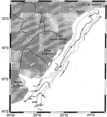
The area of study (Fig. 1) encompasses two different hydrographic regimes. The northward flow ofco1d Sub-Antarctic Waters ofthe Ma1vinasCurrent (MC) a10ng the shelf break, and the southward flow ofTropica1 Water fTomthe Brazil Current (BC) a10ng the continental margin (Emílsson, 1961; Castro Filho

et ai, 1987) (Fig. 2). The Brazil and Ma1vinas currents roeet over the continental slope off the Argentinean basin, near 36° S, creating a strong frontal zone (Gordon, 1989). Both currents then flow eastward closing the subtropical gyre. Recent descriptions of the hydrography and the circu1ationin this area have been provided by 01son et ai. (1988),

Garzoli & Garraffo (1989), Campos et aI. (1995),

and Pio1aet ai. (2000).

Data and methods

Satellite Data

The satellite-derived SST estimates are obtained fTom the Advanced Very High Reso1ution Radiometer (AVHRR) onboard the NOAA-N polar orbiting satellites. A detai1ed description of the spectral bands of the AVHRR can be found in Schwa1b(1978) and Kidwell (1991).

40"5

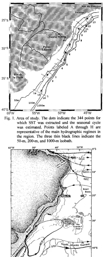
60'W 55"W 50"W 45"W Fig. 1. Area of study. The dots indicate the 344 points for

which SST was extracted and the seasonal cycle was estimated. Points labeled A through H are representative of the main hydrographic regimes in the region. The three thin black tines indicate the 50-m, 200-m, and l000-m isobath.

LENTINIet a!.: The annual cycle of SST in the WS AtIantic 95

SSTs are derived fTom Global Area Coverage (GAC) data. The spatial resolution of the AVHRR GAC data is 4 km at nadir. Global SST fields are produced at the University of Miami's Rosenstiel School of Marine and Atmospheric Science (RSMAS) using the SST estimates provided

by NOAAINESDIS (National Oceanic and

Atmospheric Administration/National Environrnental Satellite and Data lnformation Service). Sea surface temperature is computed using a multichannel algorithm (MCSST) for AVHRR infTaredchannels 4 and 5 (McClain et a!., 1985).

The MCSST is derived fTom a multiple-regression analysis using coincident satellite and drifting buoy data (Barton, 1995). The root-mean-square (rms) errarfor global estimates of SST using channels 4 and 5 is typically 0.6°C (Barton, 1995; Walton et a!., 1998). This value is simply the rms

error obtained in the linear regression analysis used to derive the MCSST algorithm.

Ocean infTared measurements may include other errar sources, such as instrumental noise, residual cloud contamination, residual calibration errors, etc. Moreover, the satellite-derived SST data include discrepancies between the ocean skin temperature measured by the AVHRR and the underlying mixed layer or bulk temperature measured by the drifting buoys (Walton et aI.,1998). A current status on the accuracy of satellite-derived SST can be found in Casey & Cornillon (1999). SST fields are then mapped to a fixed earth-based grid using a cylindrical equi-rectangular projection. This grid, with element size of 18 x 18 km, has dimensions of 2048 (longitude) x 1024 (latitude) (Olson et aI.,

1988). Daytime-only cloud-fTee SST retrievals are pooled at weekly intervals. Cloudiness associated with warm westem boundary currents is a major problem for infTaredSST determination, either by not allowing SST retrievals when pixels are totally cloud-covered ar by introducing negative bias in SST estimates for cloud-contaminated pixels (Podestá et a!.,1991). Pooling them at weekly intervals increases the number of cloud-fTeepixels on an image and, at the same time, reduces the likelihood of negative bias due to cloud contamination. Description and details of the method can be found in Olson et a!.(1988). The weekly SST fields are the basis of ali subsequent analysis. The data used here is fTom radiometers onboard NOAA-7 to NOAA-13.

Aualysis

Sixteen transects defined over the area of study are considered. Out of these transects, 13 are cross-shelf and 3 along-shelf. For each transect the grid points are spaced by 25 km. The transects are oriented fTomsouth to north, and fTomonshore to the 1000-m isobath. SST values are extracted at each grid point. After the extractions, 344 individual time series

are obtained. The SST time ser'ies analyzed span 13 years, fTomJanuary 1982 to Oecember 1994.

The central premise of ali subsequent analysis is that each weekly SST series, Y(t), can be considered as the sum of several components that are distinguished by the way they vary in time. Following the nomenclature proposed by Cleveland et a!.

(1983), SST series can be mathematically expressed as

(1)

for (t = 1...N),and where: Y(t) is the observed SST value at dayt, Ttis the trend component, associated with the low-fTequencybehavior in the leveI of Y(t)

series, St is the seasonal component, a pattern that nearly repeats itself every 12 months, and it. the irregular component which describes the remaining variation. This last component can be a misnomer, since itmay contain regular pattems not captured by the other two components.

The seasonal component in each SST time series is mode1ed following the methodology described by Wyrtki (1965) and Podestá et aI.

(1991). The methodology combines the use of a general linear model to explicitly model the annual seasonal component (Cleveland et a!., 1983). The seasonal cycle of SST at each grid point was, then, modeled as a sum of sine and cosine terms representing the contribution of annual and semiannual harmonics plus a mean value. This model can be written as

Y(t)=ao+Ia}cos(hjt/365.25) +b,sin (hift/365.25)] +e(t).

)=\

(2)

where: Y(t)is the SST value at day t (expressed in days after 1 January 1982), ao is the estimated temporal mean value, aj and bj are the estimated regression coefficients for the annual harmonic, a]

and b] are the coefficients for the semiannual harmonic, and e(t) is the error term, assumed to be independent and normal1ydistributed.

The model includes only annual and semiannual harmonics because both are found to be of importance in other studies of temperature cycles in tropical (Wyrtki, 1965; Merle et aI., 1980) and subtropical (Podestá et a!., 1991; Provost et a!.,

1992) oceans. Some advantages of this model can be stated as follows: (i) data are implicitly a ftrnction of time; (ii) SSTs do not have to be observed at regular temporal intervals; and (iii) the coefficientsa(haj ...

the amount of solar irradiance on the sea surface, which are known to play the major role in forcing the annual SST cycle mainly in coastal and shelf seas, have a sinusoidal pattem (Seckel & Beaudry, 1973).

To evaluate the adequacy of the model, the

F-statistic is calculated. For a review of the method, the reader is referred to Brook & Amold (1985). The goodness of the model can be expressed through the coefficient of determination (,-2 ), which, in turn, measures the proportion of the variation in y that is explained by the predictor variables(x).

Results

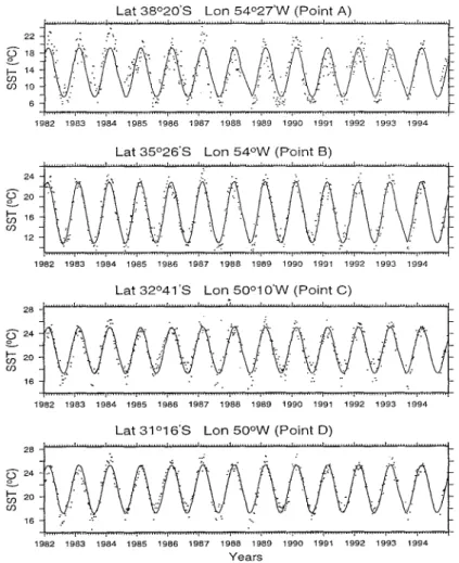
Due to the large amount of regressions performed, it is decided to select eight points as representatives of the main oceanographic features for further analyses. Point A (J8°20'S, 54°27'W) js influenced by the offshore extensions of both Brazil and Malvinas currents, Point B (35°26'S, 54°W) is approximately on the midshelf off Rio de Ia Plata,

Point C (34°41'S, 5001O'W) is located in Brazil Current waters, Points D (31°16'S, 50'W) and F (26°31'S, 4TO1'w) are on the mid-outer shelf, Points E (29°41'S, 49°W) and H (24~3' S, 45°08'W) are on the midshelf, and finalIy Point G (25°56'S, 45°20'W), which is influenced offshore by the meandering partem ofBrazil Current. The estimated SST seasonal cycle tracks the observed SST quite welI, suggesting that the sinusoidal model (Eq. 2) is adequate (Figs 3 and 4).

Overall significance of the fitting

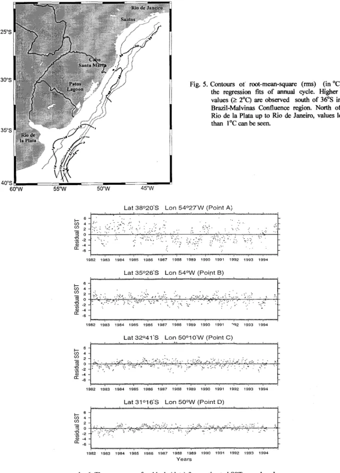
For the 344 time series, the regression model is significant. In every case, the probability of the overalI F-test is <0.01. The high significance of the regression model suggests that the selected model accounts for most of the variability in SST distributions. As an index of the model fit, thermsof the residuaIs for alI grid points is l.l7°C with a range ofO.80° to 2.69°C (Fig. 5).

Lat 38°20'8 Lon 54°27'W (Point A)

22

2:18 f- 14 (f)

(f) 10

1982 1983 1984 1985 1986 1987 1988 1989 1990 1991 1992 1993 1994

24

~

20

tn

16 (f)

12

1982 1983 1984 1985 1986 1987 1988 '989 1990 1991 1992 1993 1994

28

Lat 32°41 '8 Lon. 50°1 O'W (Point C)

1982 1983 1984 1985 1986 1987 1988 1989 1990 1991 1992 1993 1994

28

Lat 31°16'8 Lon 500W (Point O)

~

24

tn

20 (f)

16

1982 1983 1984 1985 1986 1987 1988 1989 1990 1991 1992 1993 1994 Years

LENTINIet ai.: The annual cycIe of SST in the WS AtIantic 97

28

Lat 29°41 '8 Lon 49°W (Point E)

~

24

~ 20

(j)

16

1982 1983 1984 1985 1986 1987 1988 1989 1990 1991 1992 1993 1994

30

Lat 26°31'8 Lon 47°01'W (Point F)

-

26

~

I- 22 (j) (j)

18

1982 1983 1984 1985 1986 1987 1988 1989 1990 1991 1992 1993 1994

28

Lat 25°56'8 Lon 45°20'W (Point G)

~

I- 24 (j) (j)

20

1982 1983 1984 1985 1986 1987 1988 1989 1990 1991 1992 1993 1994

30

Lat 24°23'8 Lon 45°0S'W (Point H)

-

26

~

I- 22 (j)

(j) ,

-18

1982 1983 1984 1985 1986 1987 1988 1989 1990 1991 1992 1993 1994

Years

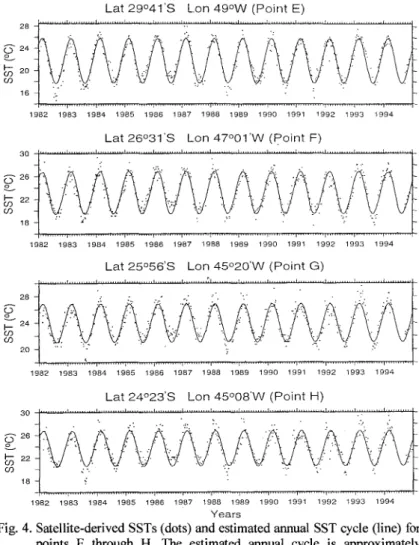
Fig. 4. Satellite-derived SSTs (dots) and estimated annual SST cycIe (line) for points E through H. The estimated annual cycIe is approximately symmetric with maxima and minima SSTs observed about six months apart reflecting a pattem typical of midlatitudes.

Variance in SST values explained by the sinusoidal fit is quantified by the coefficient of determination (?). The spatial distribution of

?

is shown in Figure 8.

Although the r2 values are probably slightly overestimated due to serial correlation, emphasis should be placed on the spatial pattem and the relative magnitudes as discussed by Chelton (1983) and Podestá et aI. (1991). From south of Rio de Ia Plata estuary up to 28° S, the coefficient of determination is highest (?>90%) on the continental shelf. In the BMC region and north of25°S, low values (? < 80%) are observed offshore and onshore, respectively, reflecting large rms

values(~ 2°C). These large values are probably due

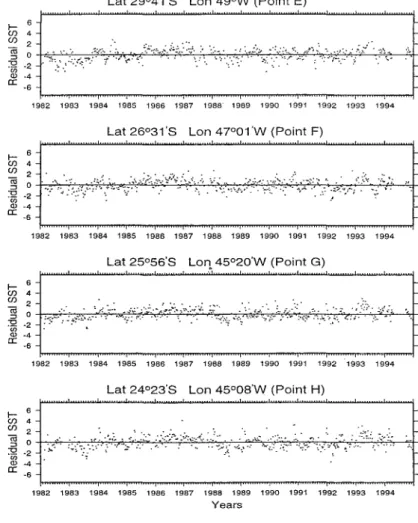
to advective processes related to meridional displacement and eddy shedding ffom the BC in the BMC, and the strong meandering of the BC north of 25°S. These processes introduce SST variabilities that are not directly associated with the seasonal cycle. Points A, G, and H are representative of these two hydrographic features, clearly seen in the residual plots by the scattering of residuaIs around the adjusted values (Figs 6 and 7).

The closeness of point H to the well-known upwelling region south of Cabo Frio (RJ) (Castro Filho & Miranda, 1998) is also reflected in the SST residual plot. Negative SST residuaIs mostly observed during austral spring-summer season, when upwelling favorable conditions prevail (Valentin et ai., 1987), are suggestive of this scenario.

The seasonal cycle

Fig. 5. Contours 01"root-mean-square (rrns) (in 0c) of the regression fits of annual cycle. Higher rrns values (~ 2°C) are observed south of 36°S in the Brazil-Malvinas Confluence region. North of the Rio de Ia Plata up to Rio de Janeiro, values lower than 1°C can be seen.

Lat 38°20'8 Lon 54°27'W (Point A)

6 t:; 4

(f) 2 ~ o ~ .2

Q) -4 tI: -6

, .

,', ';.: ".".

..' ..

'. .:~'.

:.:. :.;' ..;.-; -,

. .~ ::. . .

&;.-. .

:,' .. ~ o'... .'

'. _.'

1982 1983 1984 1985 '986 1987 1988 1989 1990 1991 1992 1993 1994

Lat 35°26'8 Lon 54°W (Point B)

.:-::;-- =.::;., :>:- ~~ .:../.,~ ..;.. .."_{.: .~~ :'.'/ ::}: ~ . .!:::."-::-:: : ,.,.

,....

.,

1982 1983 1964 1985 1986 1987 1988 1989 1990 1991 '"IQ2 1993 1994

Lat 32°41'8 Lon 50°1 o'W (Point C)

6

t:; 4

(f) 2

~

o

~

~~

tI: -6

I :"'::.::' .~_:...~. .::.~~~,: \:::~:~.::~? : ~;~;..,~:~,:::' ::~~. ': ~:~:.- '.'

1982 1983 -1984 1985 1986 1987 1988 1989 1990 1991 1992 1993 1994

Lat 31 °16'8 Lon 500W (Point D)

6 t:; 4

(f) 2 ~ o

~

~~

tI: -6

..._.;> 0.° .:.~: "._0 ",:: n

::_:.',' ' 1;. ':" ::...

1982- 1983 1984 1985 1986 1987 1988 1989 1990 1991 1992 1993 1994 Years

LENTlNIet aI.: The ann~ cycle of SST in the WS Atlantic 99

The resulting distribution of the mean estimated SST for the austral summer (JFM) and the austral winter (JAS) shows the basic large-scale temperature structure for the region of study (Figs 9 and 10). Estimated surface water temperatures during summer show small cross-shelf thermal gradients. The whole shelf has essentially homogeneous temperatures. From Rio de Janeiro to the mean latitude of separation of the Brazil Current ttom the continental margin (Olson et ai.,

1988), the region is dominated by the southward flow of BC warm waters, with surface temperatures higher than 20°C. Although local heating is known to be an important factor, the orienmtion of the isotherms suggests that an increase in surface temperature is primarily due to the advection of warm waters ttom lower latitudes. In winter, however, minimum temperatures tend to be parallel to the coast and a strong thermal gradient devt<lops offshore (Fig. 10). In this season, subantarctic cold waters reach their northernmost position, occupying most of the continental shelf portion south of the Patos Lagoon, with surface temperatures ranging

between 7°C and 14°C. North of 32°S, a strong thermal contrast (> 3° C) over the shelf-break can be observed. The southernmost limit ofBC is typically marked by average temperatures higher than 18°C, extending ttom shelf to slope regions. However, one has to keep in mind that this is only a surface feature, not totally coincident with the sub-surface and deeper circulations.

Amplitude afthe Seasonal Cycle

The estimated coefficients for the seasonal model are used to compute the highest and the lowest SST values for each grid point and the day of the year at which they will occur. The amplitude of the annual cycle is calculated as the maximum minus the minimum predicted SST. Generally, the annual amplitude (in 0c) of the sinusoidal model (Eq. 2) is maximum on the shelf. The general tendency is an amplitude decrease ttom south to north and &om inshore to offshore, reaching values higher than 7°C on the shelf (Fig. 11).

Lat 29°41'8 Lon 49°W (Point E)

1982 1983 1984 1985 1986 1987 1988- 1989 1990 1991 1992 1993 1994

Lat 26°31'8 Lon 47°01'W (Point F)

6 ti:; 4 (/) 2

~ o -o -2 .~ -4 a: -6

1982 1983 1984 1985 1986 1987 1988 1989 1990 1991 1992 1993 1994

Lat 25°56'8 Lon.45°20'W (Point G)

6 ti:; 4 (/) 2

~ o

~

~~

a: -6

1982 1983 1984 1985 1986 1987 1988 1989 1990 1991 1992 1993 1994

Lat 24°23'8 Lon 45°0S'W (Point H)

...

1982 1983 1984 1985 1986 1987 1988 1989 1990 1991 1992 1993 1994 Years

(Podestá et aI., 1991). Small variations in SST amplitude occur further north and away from the shelf-break (> 7"C), where the region is mostly dominated by warm waters of the Brazil Current throughout the year.

40"8

60"W 55"W 50"W 45"W

Fig. 8. Contours of the coefficient of determination (r2 x ] 00) of the regression fits of annual cycle. Values are expressed as percentages. High r2 values (> 90%) are near the coast, where the adjusted model tracks better the observed SSTs.

35"8

40"8

60"W 55"W 50"W 45"W

Fig.9. Estimated maxima annual SSTs at each grid point (in "C) for austral summer (Jan-Feb-Mar).

The largest annual amplitudes (12-13"C) occur otl Rio de Ia Plata estuary, where depths range from 20 to 200 meters. On the shelf, amplitudes range from I I"C south of 33"S to 6"C north of 30"S. Offshore, maximum amplitudes (10-II "C) are observed in the area of MC recirculation

35"8

40"8

60"W 55"W 50"W 45"W

Fig. 10. Estimaled minima annual SSTs aI each grid point (in "c) for austral winter (Jul-Aug-Sep).

30"8

35"8

40"8

60"W 50"W 45"W

Fig. 13. AmpJitude of lhe annual SST cycle, estimated as the difference between the highest and lowest predicted SSTs at each grid point. The amplitude decreases offshore, and the highest amplitude is observed off Rio de Ia Plata.

30"8 , /1: 25"8

1I

35"8

LENTINIet ai.:The annual cycle of SST in the WS Atlantic 101

Timing of the seasonal cycle

Figures 12 and 13 show the day of the year when maxima and minima predicted SSTs occur. On the shelf, the general tendency for the phase of the maximum annual SST referred to January I is between 30 days (at the mouth of Rio de Ia Plata estuary) and 70 days (in the South Brazil Bight and in the BC flow region). Most of the area, however, experiences the highest temperatures between days 50 and 70, which corresponds to February (19) and March (11),

respectively. In Figure 12, the timing of maximum predicted SST is between days 30-40 south of 35°S and wet of 55°W at the mouth of Rio de Ia Plata estuary, and is between 60-70 days north of 34°S and east of 50oW, extending from the coast to 1000 m offshore.

Generally, south of Cabo de Santa Marta the region warms up quicker than north of this boundary, reaching higher predicted temperatures in February than the beginning of March. This implies that the highest summer surface temperatures can be reached approximately 30 days earlier in the southern portion and inshore of BC domain.

Fig. 12. Day of the year (starting from January jSt) in which maximum SST is predicted to occur. Most of the are a experiences the highest surface temperatures between 50 and 70 days, which corresponds to February (19) and March (lI), respectively.

Fig. 13. Day of the year (starting from January jSt) in which minimum SST is predicted to occur. The predicted days of minima SSTs range from the beginning of August (8) to the beginning of September (7).

The predicted days of minimum temperature range from the beginning of August (day8) to the beginning of September (day 7). These values correspond to two regions: north of the Patos Lagoon and on the shelf; off the 200-m isobath and south of the Patos Lagoon. The temporal lag for minimum predicted SSTs is less than that for maximum predicted SSTs.

Discussion

represent the SST annual cycle. The seasonal cycle accounts for more than 90% of total SST variability. SST variations within a year clearly show the existence of distinct seasons. The adjusted annual SST cycle can be considered as approximately symmetric with minima and maxima surface temperatures observed about six months apart. This sinusoidal pattem, typical of midlatitudes, suggests that SST is forced mostly by seasonal fluctuations in solar radiation (Seckel & Beaudry, 1973). For tropical and subpolar latitudes, however, the semiannual component is as important as the annual component, giving an asymmetrical pattem to the seasonal SST cycle (Merle et a/., 1980; Provost el aI.,1992).

The model, thus, allows the reconstruction of an SST field for any day of the year by using the regression coefficients from the sinusoidal model (Eq. 2) with an accuracy greater than 1.0°C on the inner and mid-shelf regions. Small variances of the predicted SSTs are near the coast, where the adjusted model tracks better the observed SSTs (see Fig. 6). The small variance at points where residuaIs are large, like in the frontal region (e.g., point A), indicates that although signals with other periods are important there, the annual cycle is undoubtedly clearly defined.

Although a sinusoidal cycle with a single annual frequency'Seems to explain accurately most of the temporal variations of the SSTs, one can easily distinguish other periodic signals in the residual time series. The characterization of the SST annual cycle estimated here may be affected by long-term trends, obviously not completely resolved by thirteen years of data. For instance, analysis of the SST residuais (not shown here) do not suggest any significant upward trend as the one reported by Strong (1989). Instead, the oscillations of the residuaIs from the annual cycle about the zero line are more indicative of a low-frequency component of SST variability than any other long-term trend. Indeed, such interannual variability is known to exist, as reported by recent in situ and satellite-based observations in the WSA (Campos et a/., 1996; Diaz et a/., 1998; Stevenson

et a/., 1998; Campos et a/., 1999; Lentini et a/.,

2001). These studies describe the occurrence of important non-seasonal SST features appearing within a few years of each other. Using the same dataset described here, after the removal of the seasonal cycle Lentini et aI. (op. cit.)observe a total of thirteen cold and seven warm SST anomalies during and right after ENSO onset in the area of study.

As a consequence, these SST anomalies radically change the local physical (Campos et a!.,

1996; Lentini et a/., op. cit.)and biological dynamics (Bakun, 1993; Stevenson et aI., 1998; Sunye & Servain, 1998) in the WSA continental shelf For a compact description of the occurrence of these SST

anomalies in the area of study the reader should refer to Lentini et aI. (op. cit.).

Podestá et aI. (1991) compared the estimated annual cycle with the COADS climatology for the Southwestem Atlantic. Even though the predicted SST map was on aio square grid, the spatial structure of the westem boundary currents had a much more realistic appearance than the one derived from COADS dataset. Exceptions may be observed in the frontal region of BMC zone and the region affected by the Rio de Ia Plata dynamics. In the confluence region, uncertainties increase to 2.69°C offshore, probably associated to the energetic eddy field made up ofhigh amplitude meanders and detached rings and eddies (Olson et a!., 1988).

Displacement of these features may cause relatively large SST changes at a particular location not directly related to the annual cycle. Off Rio de Ia Plata the model has a relatively low accuracy of 1.5°C, probably as a consequence of the temperature differences between freshwater runoff and surface cooling to adjacent open sea surface (Piola et a/.,

2000).

, The estimated amplitude of the annual SST cycle ranges between 4°C and 13°C throughout the study area, where a southward alongshelf gradient is basically established. During summer, an increase of transport by the BC advects warm waters further south of its mean separation latitude (Olson et aI.,

1988; Matano, 1993). This seasonal increase adds up warm waters to the regular annual cycle contributing, thus, for the large amplitudes observed south off Patos Lagoon and off Rio de Ia Plata. During winter, however, the stronger Malvinas Current, 70 Sv (Peterson, 1992) against 20 Sv (1 Sv = 106m3s'1) (Gordon & Greengrove, 1986; Campos et a/., 1995),

essentially pushes the Brazil Current northward up to 300S and offshore. Coastal waters are apparently modified by surface heat fluxes over the Argentinean continental shelf and by freshwater discharge from Rio de Ia Plata (Piola et a!.,2000). South of 40° S, the shelf is dominated by excess evaporation over precipitation and continental runoff (Bunker, 1988). The region exhibits large seasonal variations associated with air-sea heat fluxes, which, in tum, drives large variations in density fields at seasonal to higher frequencies. Indeed, the combination of the north-south seasonal displacement and the large contrast between air and water temperatures (Provost

et aI., 1992) is certainly responsible for the large amplitude values observed.

LENTINIet a!.: The annual cycle of SST in the WS Atlantic 103

The region represented by point H shows a 10-day temporal lag to its surrounding. This can a1so be observed in Figure 6, where r2 values are lower than 85%. This local maximum cou1d be associated with the meandering pattem, frontal vortices pinched off the Brazil Current around Cabo Frio (RJ), anel/or upwelling-favorab1e conditions south of Cabo Frio (RJ). The spatial pattem of the predicted times of minimum SST is much more uniform than that of the maximum, which a south-north lag is observed again.

As stated by Podestá et aI. (1991), the timing for maximum and minimum SST values is sensitive to the regression coefficients used in the prediction. As the coefficients should be inflated by serial correlation, the confidence intervals should be narrow and the estimated dates would be slightly higher. The spatial pattems for both minima and maxima temperatures show a good estimative for the phase, since each data point in the grid is extraçted from weekly images.

The annual minimum SST is estimated to occur in August-September, whereas the annual maximum SST is predicted to take place in February-March. Oceanographic/meteoro10gical conditions are known to control fish distribution and abundance (e.g., Lima & Castello, 1995; Sunye & Servain, 1998). Estimates of the timing of the annual cycle, thus, can be useful to understand, the occurrence, distribution, and migration of local economic fish stocks. For example, the optimum temperature for the distribution of sardine along the Brazilian coastline is between 19°-26°C (Matsuura et aI., 1991; Saccardo & Rossi-Wongtschowski, 1991). Its spawning activity reaches a peak in austral summer, being essentially confined within the South Brazil Bight (SBB) (Bakun, 1993). Therefore, latitudinal variations in sea surface temperatures, which may serve as a good indicator of water column temperature, may be responsible for sardine migration in the SBB. As another example, the Brazilian anchovy and the Argentine hake are spatially segregated by temperature (Bakun,op. cit.).Both anchovy and hake migrations occur fTom late winter to early summer (Lima & Castello, 1995; Podestá, 1990), at the time when shelf-break waters begin to warm up.

Conclusions

1n retrospect, this paper provides a detailed description of the seasonal SST cycle in the Westem South Atlantic continental shelf. Emphasis has been placed on the spatial distribution of the timing and amplitude of the annual SST cycle. The lack of long time series of oceanographic data in the southem hemisphere makes satellite-derived SST time series over the area of study a particularly valuab1edata set. The high spatial resolution and quasi-synoptic

coverage of satellite-derived SST observations may allow meaningfu1 estimates of spatia1 and temporal pattems of SST anomalies particular1y near ocean boundaries, where their closeness to 1andmakes their influences more direct and strong. Coastal waters store the sun's heat in summer and release it to the atmosphere in winter, he1pingto moderate the climate of littoral regions. AIso, as SST anoma1ies strongly influence the coup1ing between ocean and atmosphere, the methodology presented here may contribute to an understanding of interannua1 variability related to climate change. Such an approach can be seen in Campos et aI.(1999) and Lentini et aI.(2001), where after removal ofthe SST seasonal cycle, a deep investigation of interannua1 SST variability is done.

Acknowledgements

This work. is a result of efforts supported by the Inter-American Institute for Global Change Research (IAI), through the SACC's CRN and ISP-I

Projects, by the Conselho Nacional de

Desenvolvimento Científico e Tecno1ógico (CNPq) (Proc. no. 201443/96-1), and by the Fundação de Amparo a Pesquisa do Estado de São Paulo (FAPESP) (Proc. 96/4060-0). The authors express their gratitude to O. Brown and D. 01son, fTom RSMAS/Univ. of Miami, who provided the data, part of the financia1 support and guidance for the first author during a visit to the USA, when a pre-ana1ysis of the AVHRR data set was done. We extend our appreciation to the reviewers for their valuab1e comments.

References

Bakun, A. 1993. The Califomia Current, Benguela Current, and southwestem Atlantic shelf ecosystems: a comparative approach to identifYing factors regulating biomass yields. In: Sherman, K.; Alexander, L. M. & gold, B. D. eds Stress migration and preservation of large marine ecosystems. Washington, AAAS. p. 199-221.

Barton, L 1. 1995. Satellite-derived sea surface temperatures: Current status. 1. geophys. Res., 1OO(C5):8777-8790.

Brook, R. 1. & Amold, G. C. 1985. Applied regression analysis and experimental designoNew York, M. Dekker. 237p.

Bunker, A. F. 1988. Surface energy fluxes of South Atlantic Oceano Mon. weath. Rev., 116(4):809-823.

Campos, E. 1. D.; Lentini, C. A. D.; MiIler, 1. L. & Pio1a, A. R. 1999. Interannua1 variabi1ity of the sea surface temperature in the South Brazi1 Bight. Geophys. Res. Letts, 26(14):2061-2064.

Campos, E. 1. D.; Ikeda, Y; Castro Filho, B. M.; Gaeta, S. A.; Lorenzzetti, J. A. & Stevenson, M. R. 1996. Experiment studies circu1ation in the western South Atlantic. EOS Trans. Am. geophys. Un., 77(27):253-259.

Campos, E. 1. D.; Gonçalves, 1. E. & Ikeda, Y. 1995. Water mass characteristics and geostrophic circu1ation in the South Brazi1

Bight-Summer of 1991. 1. geophys. Res.,

100(Cll):18537-18550.

Casey, K. S. & Comillon, P. 1999. A comparison of satellite and in-situ-based sea surface temperature c1imatologies.1. Climate,

12(6):1848-1863.

Castro Filho, B. M. & Miranda, L. B. 1998. Physical

oceanography of the western Atlantic

continental shelf located between 4°N and 34°S costal segment (4'W). In: Robinson, A. R. & Brink, K. H. The Sea. Oxford, John Wiley & Sons. p.209-25I.

Castro Filho, B. M.; Miranda, L. B. & Miyao, S. Y 1987. Condições hidrográficas na plataforma continental ao largo de Ubatuba: variações sazonais e em média escala. Bolm Inst. oceanogr., S Paulo, 35(2):135-151.

Chelton, D. B. 1983. Effects of samp1ing errors in statistical estimation. Deep-Sea Res., 30(10): 1083-1103.

Cleveland, W. S.; Freeny, A. E. & Graedel, T. E. 1983. The seasonal component of atmospheric COz

-

Information IToma new approaches to the decomposition of seasonal time series. J. geophys. Res., 88(CI5):10934-10946.

Diaz, A. F., Studzinski, C. D. & Mechoso, C. R. 1998. Relationships between precipitation anomalies in Uruguay and Southern Brazil and sea surface temperature in the Pacific and Atlantic Oceans. 1. Climate, II (2):251-271.

Emilsson, r. 1961. The shelf and coastal waters off southem Brazil. Bolm Inst. oceanogr., S Paulo,

11:101-112.

Gacic, M.; Marullo, S.; Santoleri, R. & Bergamasco, A. 1997. Analysis of the seasonal and interannual variabi1ity of the sea surface temperature field in the Adriatic Sea fi-om AVHRR data (1984-1992). J. geophys. Res., 102(C 10):22937-22946.

Garzo1i, S. L. & Garraffo, Z. 1989. Transports, Frontal Motions, and Eddies at the Brazil-Malvinas Currents Confluence. Deep-Sea Res., 36(5A):681-703.

Gordon, A. L. 1989. Brazil-Malvinas confluence 1984. Deep-Sea Res., 36(3A):359-384.

Gordon, A. L. & Greengrove, C. L. 1986. Geostrophic circulation of the Brazil-Falk1and Confluence. Deep-Sea Res., 33(5A):573-585.

Hore1, 1. D. 1982. On the annual cyc1eof the tropical Pacific atmosphere and oceano Mon. Weath. Rev., 110(12):1863-1878.

Kidwell, K. B. 1991. NOAA Polar Orbiter Data User's Guide (TIROS-N, NOAA-6, NOAA-7, NOAA-8, NOAA-9, NOAA-10, NOAA-ll, and

NOAA-12). Washington, NOAA/NESDIS

Satellite Data Services Division, De.

Lentini, C. A. D.; Podestá, G. P.; Campos, E. 1. D. & 0lson, D. B. 2001. Sea surface temperature anomalies on the westem South Atlantic fi-om

1982 to 1994. Continent. Shelf Res. 21(I ):89-112.

Lima, r. D. & Castello, 1. P. 1995. Distribution and abundance of South-west Atlantic anchovy spawners (Engraulis anchoita) in relation to oceanographic processes in the southem Brazilian shelf. Fish. Oceanogr., 4(1):1-16.

Matano, R. P. 1993. On the separation of the Brazil Current fi-om the coast. 1. phys. Oceanogr., 23(1):70-90.

Matsuura, Y.; Spach, H. L. & Katsuragawa, M. 1991. Comparison of spawning pattems of the Brazilian sardine (Sardinella brasiliensis) and anchoita

(Engraulis anchoita)in Ubatuba Region, Southern Brazil during 1985 through 1989. ICES C. M., H22. 25p.

McClain, E. P.; PicheI, W. G. & Walton, C. C. 1985. Comparative performance of AVHRR-based multichannel sea surface temperatures. 1. geophys. Res., 90(C6):11587-11601.

LENTINIet a!.: The annual cycIeafSST in the WS Atlantic 105

Olsan, D. 8.; Podestá, G. P.; Evans, R H. & Brown, O. 8. 1988. Temporal variations in the separation of Brazil and Malvinas Currents. Deep-Sea Res., 35(12): 1971-]990.

Peterson, R. G. ]992. The boundary currents in the westem Argentine Basin. Deep-Sea Res., 39(3-4A):623-644.

Peterson, R G. & Stramma, L. ]991. Upper-Ievel circulation in the South Atlantic. Ocean Prog. Oceanogr.,26(]):]-73.

Piola, A. R.; Campos, E. J. D.; Mõller, O. O.; Charro, M. & Martinez, C. 2000. The subtropical shelf ffont off eastem South America. J. geophys. Res.,

]05(C3):6565-6578.

Podestá, G. P.; O. 8. Brown & Evans, R H. ]991. The annual cycle of satellite-derived sea surface temperature in the Southwestem Atlantic Oceano J. Climate, 4(4):457-467.

Podestá, G. P. ] 990. Migratory pattem of Argentine hake (Merluccius hubbisi) and oceanic processes in the southwestem Atlantic Oceano Fish. BulI., 88(1):]67-]77.

Provost, c.; Garcia, O. & Garçon, V. 1992. Analysis of satellite sea surface temperature time series in the Brazil-Malvinas Current Confluence region: dominance of the annual and semiannual periods. J. geophys. Res., 97(C] ]):1784]-]7858.

Saccardo, S. A. & Rossi-Wongtschowski, C. L. D. 8. ]991. Biologia e avaliação do estoque de sardinha

Sardinella brasiliensis: uma compilação. Atlântica, Rio Grande, 13(1):29-43.

Schwalb, A. ]978. The TIROS-NINOAA A-G

satellite series. NOAA Tech. Memo. NESS 95, p.75.

Seckel, G. R. & Beaudry, F. H. ] 973. The radiation ffom sun and sky over the North Pacific Oceano Trans. Am. geophys. Un., 54(1]):]] ]4.

Stevenson, M. R; Dias-Brito, D. D.; Stech, J. L. & Kampel, M. ]998. How cold water biota arrive in tropical bay near Rio de Janeiro, Brazil? Continent. ShelfRes., ]8(13):]595-1612.

Strong, A E. ]989. Greater global warming revealed by satellite-derived sea surface temperature trends. Nature, 338(62] 7):642-645.

Strub, P. T.; Allen, J. S.; Huyer, A; Smith, R L. & Beardsley, R C. 1987. Seasonal cycles of currents, temperatures, winds, and sea levei over the northeast Pacific continental shelf: 35"N to 48°N. J. geophys. Res., 92(C2):1507-]526.

Sunye, P. S. & Servain, J. ]998. Effects of seasona] variations in meteorology and oceanography on the Brazilian sardine fishery. Fish. Oceanogr., 7(2):89-] 00.

Valentin, J. L.; Andre, D. L. & Jacobs, S. A ]987. Hydrobiology in the Cabo Frio (Brazi]) upwelling: two-dimensional structure and variability during a wind cycle. Continent. She]f Res., 7(1):77-88.

Walton, C. c.; Pichei, W.G.;Sapper, J. F. & May, D. A. ]998. The development and operationa] application of nonlinear algorithms for the measurement of sea surface temperatures with the NOAA polar-orbiting environmental satellites. J. geophys. Res., ]03(C]2):27999-280]2.

Wyrtki, K. 1965. The annual and semiannual variation of sea surface temperature in the North Pacific Oceano Limnol. Oceanogr., ]0(3):307-3 ]]0(3):307-3.