STUDY OF THE EQUATORIAL ATLANTIC OCEAN MIXING LAYER USING A
ONE-DIMENSIONAL TURBULENCE MODEL*
Udo Tersiano Skielka1,**, Jacyra Soares1 and Amauri Pereira de Oliveira1
1Universidade de São Paulo – Instituto de Astronomia, Geofísica e Ciências Atmosféricas
Departamento de Ciências Atmosférica (Rua do Matão 1226, 05508-900 São Paulo, SP, Brasil)
**Corresponding author: [email protected]
A
B S T R A C TThe General Ocean Turbulence Model (GOTM) is applied to the diagnostic turbulence field of the mixing layer (ML) over the equatorial region of the Atlantic Ocean. Two situations were investigated: rainy and dry seasons, defined, respectively, by the presence of the intertropical convergence zone and by its northward displacement. Simulations were carried out using data from a PIRATA buoy located on the equator at 23o W to compute surface turbulent fluxes and from the
NASA/GEWEX Surface Radiation Budget Project to close the surface radiation balance. A data assimilation scheme was used as a surrogate for the physical effects not present in the one-dimensional model. In the rainy season, results show that the ML is shallower due to the weaker surface stress and stronger stable stratification; the maximum ML depth reached during this season is around 15 m, with an averaged diurnal variation of 7 m depth. In the dry season, the stronger surface stress and the enhanced surface heat balance components enable higher mechanical production of turbulent kinetic energy and, at night, the buoyancy acts also enhancing turbulence in the first meters of depth, characterizing a deeper ML, reaching around 60 m and presenting an average diurnal variation of 30 m.
R
E S U M OO modelo General Ocean Turbulence Model (GOTM) é aplicado para diagnosticar o campo de turbulência da camada de mistura oceânica (CM) na região equatorial do Oceano Atlântico. Foram investigadas as estações chuvosa e seca, definidas, respectivamente, pela presença da zona de convergência intertropical e pelo seu deslocamento para norte. Simulações foram realizadas usando dados da bóia PIRATA (0o, 23oW) para o cálculo dos fluxos turbulentos de superfície e dados do
Projeto NASA/GEWEX Surface Radiation Budget para “fechar” o balanço de radiação na superfície. Um esquema para assimilação de dados foi usado para considerar os mecanismos físicos não representados pelo modelo unidimensional. Para a estação chuvosa, os resultados mostraram uma CM rasa devido à menor tensão de cisalhamento na superfície e a estratificação estável da camada superior oceânica; a profundidade máxima alcançada é da ordem de 15 m com uma variação diurna média de 7 m de profundidade. Na segunda estação, a tensão de cisalhamento mais intensa e o aumento das trocas de calor em superfície geraram maior produção mecânica de energia cinética turbulenta e a noite o empuxo também favoreceu a formação de uma CM mais profunda, alcançando até 60 m, e com variação diurna de 30 m em média.
Descriptors: Oceanic turbulence, General Ocean Turbulence Model, Equatorial Atlantic Ocean, Turbulent kinetic energy.
Descritores: Turbulência oceânica, Modelo geral de turbulência oceânica, Oceano Atlântico equatorial, Energia cinética turbulenta.
I
NTRODUCTIONThe equatorial ocean is distinct from other oceanic regions due to its dynamic and thermodynamic particularities. Approaching the equatorial region, the geostrophic balance diminishes
__________
(*) Paper presented at the Symposium on Oceanography, 4., 2008, São Paulo, IOUSP.
regions, the annual variations of the sea surface temperature (SST) are the dominant cycle and depend more on oceanic and air-sea interaction processes than on the annual cycle of the surface heat fluxes (Carton and Zhou, 1996; Yu et al., 2006 for the tropical Atlantic Ocean), prevailing variations of wind-induced vertical mixing, vertical and horizontal advection of heat (Weingartner and Weisberg, 1991a) and wind driven cooling due to evaporation, which is related to ocean-atmosphere feedback processes (e.g. Carton et al., 1996; Chang et al., 2000). All these processes are, direct or indirectly, related to the surface wind relaxation and strengthening that is determined, in great part, by the seasonal displacement of the intertropical convergence zone (ITCZ).
The ITCZ is located over regions of warmer waters, where intense atmospheric convection and, therefore, cloudiness and heavy precipitation exist (e.g. Hasthenrath 1991). When the ITCZ is located over a certain region, horizontal wind intensity weakens and cloudiness decreases the major components of the radiation surface balance. Despite the reduction in the incoming solar radiation at the surface, previous studies have identified the role of wind relaxation in promoting the increase in the SST as the result of two main factors: reduction of the wind-induced latent heat loss and the rise of the thermocline. This last factor is a non-intuitive mechanism, but as the thermocline approaches the surface it becomes easier to entrain cold water in the surface layer and thus decrease the SST. However, observational studies over the equatorial region have evidenced that sudden wind relaxation over the basin scale promotes a rapid cessation of the turbulent mixing, decoupling the mixing layer (ML) from the thermocline. Accordingly, observational studies of the equatorial Atlantic Ocean from the Seasonal Response of the Equatorial Atlantic program - SEQUAL (Weingartner and Weisberg 1991a,b; Weisberg and Tang 1987), indicate that the ML responds rapidly to the strengthening and weakening of the surface winds in the equatorial region. Weingartner and Weisberg (1991a), using measurements of temperature and velocity at the equator at 28o W, showed that the uncoupling of the ML due to wind relaxation occurs in the middle of December and traps the net surface heat flux (Qn) in a thin upper layer, promoting during the
following months a highly stable surface layer. This stable condition remains and is responsible for the progressive warming of the shallow ML until late April/early May when, with the strengthening of the wind, the upwelling movement and the mixing in the ocean are consequently turned on. From May on, the SST drops mainly due to the upwelling and zonal transport of cold water from the east. This drop in temperature is counterbalanced by transient eddies triggered by tropical instability waves, whose activity
is more intense in June and July. In early August, the activity of the tropical instability waves diminishes and the cooling of the water due to advection ceases. In this period, the thermocline is deeper and attains a balance with the surface wind stress. From August to November, this state of equilibrium is maintained and the water temperature and salinity variations are smaller. The authors point out that during this period, one-dimensional mixing layer models might work accurately, since advection is less important and the surface heat fluxes seem to balance the turbulence mixing at the base of the ML.
More recently, Yu et al. (2006), using the dataset from OAFlux (Objectively Analyzed Air-Sea Fluxes, Yu et al., 2008), the ISCCP (International Satellite Cloud Climatology Project, Zhang et al., 2004) and the WOA (World Ocean Data, Levitus et al., 1994), estimated the correlation of the local variation of SST and the mixing layer depth (hMLD)
with Qn. They verified at the equator, westward from
20o W, that the rise in the SST is characterized by the mechanism described by Weingartner and Weisberg (1991a), since a negative correlation between the variation of SST and the hMLD was indentified (the
reduction of hMLD being related to an increase in SST,
and vice-versa), while eastward of 20o W, a strong
positive correlation appears due to the known upwelling region off the African coast, where the depth of the thermocline responds directly to the strengthening of the easterlies. There, the easterlies transport the surface water away from the coast, promoting upwelling, which is related to the rise of the thermocline and the decrease in the SST.
The main goal of the present study is to investigate the extent of the turbulence of the equatorial Atlantic mixing layer using the General Ocean Turbulence Model (GOTM, Burchard et al. 1999). The version of GOTM used here is based on the k-ε equations with the second-order turbulence closure scheme proposed by Canuto et al. (2001). This type of model has been tested and used in many studies of the upper ocean mixing layer (e.g. Burchard and Bolding, 2001; Bolding et al., 2002; Jefrey et al., 2008) and permits that the turbulence properties such as turbulent viscosity, tracer diffusivity, turbulent kinetic energy (TKE), dissipations rate of TKE, and others, be calculated.
The numerical simulations analyzed here will correspond to two periods: (i) February to April, when the ITCZ is over the region investigated – hereafter called Season 1 - and (ii) August to October, when the ITCZ is displaced northward – called Season 2.
The data utilized in this study are described in section 2. The second-order turbulent closure model with k-ε equations and the data assimilation are discussed in section 3. To consider realistic equatorial
features of the mean variables, oceanic in situ data from Prediction and Research Moored Array in the Tropical Atlantic (PIRATA) are assimilated to the GOTM. Section 4 presents the results and discussion and the conclusions are given in section 5.
M
ATERIAL ANDM
ETHODSData and Region Investigated
The site chosen for this study is located at (0o, 23 W), where a PIRATA buoy (henceforward identified as B23W) is moored. This buoy is part of the PIRATA’s backbone and has a long data series of the variables (Bourlès et al., 2008). It is the only buoy of the PIRATA array which has Acoustic Doppler Current Profile (ADCP) measurements, which is essential to account for the shear imposed by the EUC. Table 1 shows the different dataset used.
To compute the atmospheric turbulent fluxes at the surface – latent (Qe) and sensible (Qh) heat
fluxes and the components of wind stress (τx and τy) -
the algorithm of the Coupled Ocean-Atmosphere Response Experiment (COARE) was used. It is based on aerodynamic bulk formulae and transfer coefficients obtained from the Monin-Obukhov Similarity Theory (Fairall et al., 2003) and it requires only information about air temperature and relative humidity, wind speed and SST (Table 1). The interface parameters were computed from 10 min averaged variables extracted from the PIRATA website. The corresponding turbulent fluxes were averaged hourly, resulting in hourly time series from 2000 to 2006, with some gaps. From these hourly series, hourly climatological series were computed. This
climatological time series was used in the model simulations for Seasons 1 and 2.
Since the PIRATA array measures only the downward solar radiation (recently, PIRATA started measuring upward longwave radiation, but the data series of this variable is not as long as that of the downward shortwave radiation), data from the NASA Langley Research Center Atmospheric Sciences Data Center NASA/GEWEX Surface Radiation Budget Project (SRB) (http://gewex-srb.larc.nasa.gov) were used to close the surface radiation balance: the surface albedo, necessary to prescribe the shortwave surface balance (I0), and the longwave surface balance (Qb).
The SRB estimated many radiative parameters globally with 1o X 1o resolution, from July 1983 to June 2005, using satellite products, meteorological inputs from reanalysis and radiative transfer algorithms. Studies at the Air-Sea Interaction Research Lab-USP showed close agreement between the SRB dataset and PIRATA in situ measurements (Peres, 2007). In this study a time series compatible with that of the PIRATA time series was used, from 2000 to 2005. Since the SRB has a time resolution of 3 h, the radiative data series were linearly interpolated hourly.
Figure 1 shows the climatological hourly data series obtained from observed vertical profiles. Features similar to those described by Weingartner and Weisberg (1991a,b) may be observed in Figure 1. For temperature (Fig. 1a), one may observe higher values of SST and a more highly stratified water column in Season 1. From May onwards, the rapid decrease in temperature is related to the onset of the wind. In Season 2 a more vertically homogeneous temperature is evidenced. Figure 1b shows a shallower position of the EUC, between 50 and 80 m, for Season 1, whilst in Season 2 the EUC is located deeper, below 70 m.
Table 1. Dataset used in the model run at location (0o, 23oW).
PIRATA SRB-NASA Specification on the model
Meteorological
Air temperature; Sea surface temperature;
Relative humidity; Wind components (u and v);
Downward shortwave.
Upward shortwave; Downward and upward
longwave.
Upper boundary conditions: Momentum and heat turbulent fluxes;
Surface radiation budget.
Oceanographic Temperature, salinity and
Fig. 1. Annual cycle of the vertical profiles of (a) temperature (oC) and (b) zonal velocity (m s-1). Data are hourly average
values computed for the B23W dataset from 2000 to 2006, smoothed by a 5-day running mean.
Second-order Turbulent Closure with k-ε Equations
In this study a second-order turbulent closure model is used with k-ε equations implemented in the GOTM (Burchard et al. 1999). The second-order closure coefficients used are from Canuto et al. (2001) and according to Burchard and Bolding (2001) this closure is numerically stable, computationally cheap and showed greatest accuracy in simulating ML when the results are compared with idealized and real environment cases.
Second-order closure has been shown to achieve a good compromise in simulating turbulent processes in oceanic boundary layers in many environments, since it has low computational cost and is accurate in simulating the relevant mixing processes in high Reynolds number environments.
Generally speaking, to close the mean equation system it is necessary to estimate the covariance between the turbulent variables
( )
x′w′, as described by Eq. 1:X w
x′ ′=−
ν
t ∂z (1)Where νt is turbulent viscosity and ∂zX the flow mean
gradient.
The turbulent viscosity depends on the TKE,
k, and its dissipation rate, ε, which are prognosticated
using dynamic equations, and on so-called non-dimensional stability functions (Burchard et al., 1999
and Burchard and Baumert, 1995). These stability functions contain all the information on the second-order closure and depend basically on the semi-empirical constants and the gradients of the mean flow: the shear frequency (Eq. 2) and the buoyancy frequency (Eq. 3).
( ) ( )
[
2 2]
1/2V U
S= ∂z + ∂z (2)
( )
[
1]
1/20 ρ
ρ z
g
N= − − ∂ (3)
Where (U,V) are the mean horizontal velocity components; ∂z is the vertical derivative; ρ the mean
ocean density, ρ0 the reference density, and g the
acceleration due to gravity.
The TKE equation, given by Eq. 4, is composed of the following terms: Eq. 5 is the shear or the mechanical production which depends on the shear frequency and the turbulent viscosity (νtm); Eq. 6 is the
buoyancy production/consumption and depends on the buoyancy frequency and the temperature turbulent diffusivity (νth); Eq. 7 is the vertical diffusion,
parameterized by the semi-empirical parameter called
Schimidt number (σk) and νt m
; the viscous dissipation rate of TKE (ε) is given by Eq. 8, which is a linear combination of the terms of Eq. 4 and the semi-empirical parameters cε1, cε2, cε3 and a vertical
diffusion term (Tε). Further details may be found in
Burchard et al. (1999).
ε − + + =
∂tk P B T (4)
2 S
P m
t
ν
= (5)
2 N
B h
t
ν
= (6)
( )
kT k z
m
t ∂
=ν σ−1 (7)
(
ε ε ε ε)
εε
ε c P c B c T k
t = + + −
∂ 1 3 2 (8)
Numerically, the model has a staggered Cartesian vertical grid from the bottom, z = -H, to the free surface, z=ζ, and uses a scheme centered in space and advanced in time to solve a diffusion equation. Further details may be seen in Burchard et al. (1999).
Data Assimilation and Simulation Details
An assimilation scheme was used in the mean equations in order to consider effects not represented by the one-dimensional model, such as advection, input of freshwater at surface and also the large-scale mechanisms. For example, the EUC, which is driven below the ML due to the basin-wide pressure gradient, can be given by the zonal current observations.
Expression 9 shows the assimilation term, considered in the numerical mean equations (momentum, heat and salt conservations) and it depends on the difference between the variable prognosticated by the model (X) and that actually observed (Xobs) - which is small as the correction to the
observations is performed at each time step - and after a prescribed period of assimilation (Tassim).
(
obs)
assim
tX∝−T X−X
∂ −1 (9)
The vertical resolution of the observations may be considered coarse compared to the model resolution. Usually, the vertical resolution of PIRATA observations is 5 m for current velocity, 20 m for temperature and 40 m for salinity, while the model uses 1 m as vertical resolution. Therefore, an ideal assimilation period had to be determined so that the observational time series, linearly interpolated to the model grid, would not compromise the computation of the turbulent quantities. After testing the performance of different values, an ideal Tassim of 1 day was found.
As the mean variables are well represented in the numerical model, the turbulent quantities, obtained by the model, should also be correct.
The model uses no slip and no fluxes as bottom boundary condition. Therefore, the model´s vertical domain was chosen so that the effect of the bottom would not influence the upper boundary layer simulation. The vertical domain considered for both
simulations (Seasons 1 and 2) is from z = 0 m, at the surface, to z = -200 m, in an equally spaced Cartesian grid of 1 meter. A time step of 60 s was used.
Surface Boundary Conditions
The upper boundary conditions for the model are specified in terms of the atmospheric surface fluxes of stress (τx and τy), given by Eq. 10,
and of the net heat flux, Qn, described by Eq. 11,
where Qb is the longwave surface balance, Qe is the
latent heat flux, Qh the sensible heat flux and I0 the
shortwave surface balance. Here a positive net surface heat flux corresponds to the heat gained by the ocean.
( )
uw τxρ ′ ′ =
− 0 ; −ρ
( )
v′w′0=τy (10)0 I Q Q Q
Qn= b+ e+ h+ (11)
In all simulations it was assumed that the salt flux, at the surface, was zero.
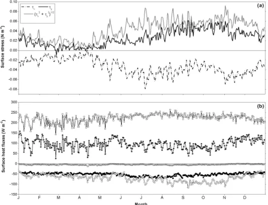
Figure 2 shows the daily averaged values computed from the hourly series used as surface boundary conditions. In Figure 2a the difference between the two seasons in relation to the atmospheric forcing is evidenced: the relaxation of the surface stress in Season 1 – with the lower values from February to the end of April - and the period of intensified winds during Season 2 – from August to the end of October.
There is low variability of the air-sea exchange at the equator during the year (Figure 2b). One can observe greater variability of the surface shortwave balance (I0, open square) in Season 1 due to
cloudiness. Despite the variability of I0, the longwave
surface balance (Qb, solid square), obtained from SRB,
does not show great variability during the year, being slightly higher in Season 2. The latent heat flux (Qe,
open circle) over the ocean depends mostly on the wind intensity, being higher during Season 2. The sensible heat flux (Qh, cross), is practically negligible,
being one order of magnitude smaller than the other terms. The resultant net surface heat flux (Qn, star),
given by Eq. 11, shows great variability throughout the year.
Table 2 shows the average values for the surface fluxes for both seasons. Season 2 presents a higher input of energy from solar radiation (difference of 28.9 W m-2), probably due to less cloud cover of the sky compared to Season 1. The main difference between the two seasons is in the cooling due to evaporation, represented by Qe. In Season 1, the
reduction in the intensity of the wind diminishes the latent heat lost at the surface (difference of 29.2 W m-2), this being the principal contributor to the higher
Fig. 2. Daily average values computed from the hourly time series. (a) Zonal stress (dashed-dotted line), meridional stress (black line) and the total stress (grey line) at surface, given by Eq. 10. (b) Components of the surface heat balance: I0 (open
square), Qh (cross), Qb (solid square), Qe (open circle) and Qn (star) given by Eq. 11.
Table 2: Mean values and standard deviations for the surface heat fluxes (W m-2) and stress horizontal components (10-2 N m-2)
for each season. I0 – shortwave surface balance; Qh – sensible heat flux; Qe – latent heat flux; Qb – longwave surface balance;
Qn – net heat flux.
τx τy I0 Qb Qe Qh Qn
Season 1 -1.4 (0.7) 0.6
(0.4) 206.7 (20.8) -48.4 (3.5) -60.7 (9.2) -5.1 (2.0)
92.5 (23.3)
Season 2 -3.8 (1.0) 4.4
(0.9) 234.6 (11.0) -56.8 (6.6) -89.9 (10.1) -5.1 (1.4)
82.9 (17.2)
R
ESULTSFor the results presented here, the first 15 days of each simulation (Season 1 and Season 2), considered as a spin up period, have been neglected. So the results presented for Season 1 refer to the period from February 15 at 00 h to April 29 at 23 h and for Season 2 from August 15 at 00h to October 30 at 23 h. Here the local time at 23o W is used. The heat gain at the ocean surface has been considered as having positive value.
Simulation Results
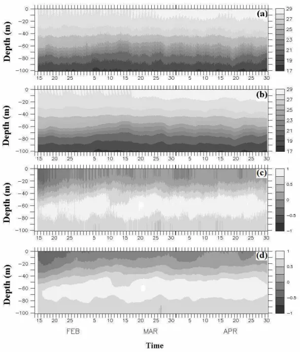
Figures 3 and 4 compare the mean field reproduced by the model with the observed data
interpolated linearly in space and time. The choice of the Tassimof 1 day attenuates the hourly variations and
therefore the data assimilation scheme allows a smooth reproduction of the main features of each season. The diurnal cycle is well reproduced with the model performing as an optimized interpolator when data are missing at some depth, as for instance, interpolating the surface zonal current, which has a predominantly westward flow (Figs 3c,d and 4c,d).
Based on these reproduced mean fields, the turbulent properties were estimated by the turbulence closure of Canuto et al. (2001).
The mean features obtained in Figures 3 and 4 agree, for both seasons, with the studies of SEQUAL on this region.
Figure 3: Time variation of (a) observed temperature, (b) reproduced temperature (0C), (c) observed zonal current and (d)
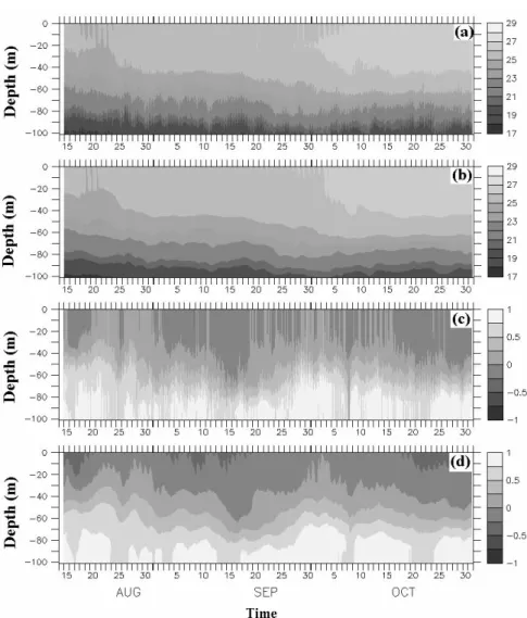
Fig. 4. Time variation of (a) observed temperature, (b) reproduced temperature (0C), (c)
observed zonal current and (d) reproduced zonal current (m s-1). Season 2.
For the period of Season 1, the highest temperature values (Fig. 3a,b), with stable stratification in the upper layer are to be observed. The EUC is located near the surface, with its core varying from 50 to 80 m (Fig. 3c,d) during Season 1.
During Season 2 the vertical temperature field is more homogeneous (Fig. 4a,b) and the EUC is located deeper, with its core positioned below 70 m. The westward momentum provided by the stronger winds is transferred down to greater depths (Fig. 4c,d). Figure 5 shows the mean density field obtained from the B23W dataset together with the
hMLD estimated by the model using a threshold value
for the TKE of 10-5 m2 s-2. According to Burchard and Bolding (2001), below this value there is insufficient energy to mix the layer.
During Season 1 (Fig. 5a) the model estimates a shallow hMLD with a restricted diurnal
variability, reaching a maximum depth around 15 m and mean diurnal amplitude around 7 m. The closed density contour lines below the upper layer indicate the great vertical stratification occurring during this season.
During Season 2 (Fig. 5b) the ML is deeper, presenting greater diurnal variability with a mean value of 30 m but reaching 60 m in early October. The ocean during this season has less vertical stratification than during Season 1.
Monterey and Levitus (1997) and Montegut et al. (2004) estimated the climatological monthly values of hMLD for this region and obtained mean
values shallower than 10 m for Season 1 and of less than 50 m for Season 2. The estimated values of hMLD,
for both seasons, are, therefore, in agreement with the climatological dataset.
The modeled hMLD accompanies the
narrowing of the density lines, which correspond to the deepening of the ML as observed, for example, in the period from February 26 to March 3 in Season 1 and from September 12 - 23 in Season 2.
Figure 6 compares the two seasons using the accumulated heat content at the surface and in the water column at different depths. The accumulated
heat was obtained at the surface by multiplying Qn by
the time step simulation and adding up the values. The accumulated heat storage in the water column was estimated by computing the heat storage rate, given by Eq. 11, and proceeding as was done for Qn, adding up
the values cumulatively.
(
∂Θ+ ⋅∇Θ)
ρ
= c h U
Qn p t (12)
Fig. 5. Density contours and the ML depth (hMLD) for (a) Season 1 and (b) Season
2. The contour interval is of 0.03 kg m-3. The thick black lines indicate the h MLD
estimated using a TKE threshold of 10-5 m2 s-2.
Fig. 6. Accumulated heat content. (a) Season 1 and (b) Season 2. For the surface heat content the computed net surface heat flux, Qn, is used as a boundary condition. The others curves correspond to the
The water column heat budget, Eq. 12, was obtained using the heat and mass conservation equation for an incompressible fluid, as shown by Moisan and Niiler (1998), where h is a depth at which the temperature is integrated from the surface; Θ is the
temperature;
U
is the mean velocity vector; cp is thespecific heat at constant pressure; ∂t is time derivative. The first term on the right-hand side is the heat storage rate integrated into the water column and the second term is the change in heat storage due to temperature advection. Despite the use of a one-dimensional model in this study, in which the advection terms of the mean equations are explicitly neglected, the assimilation scheme used here is a way of accounting for some of these effects.
The heat content at the surface varies little from Season 1 to Season 2, being slightly higher in Season 1, as is also to be observed from the values of the mean surface heat flux components (Table 2). During Season 2, despite the higher input of energy from solar radiation due to the lesser cloud coverage, the greater wind velocity increases the latent heat lost at the surface (Fig. 2). The seasonal difference between the heat content at the surface, is, therefore, due to the smaller amount of latent heat lost in Season 1.
On the other hand, during Season 1 most of the heat reaching the surface is not distributed vertically in depth, or vertically mixed (Figure 6a.) Moreover, the heat accumulated between the surface and 5 and 20 meters is less than that accumulated at the surface. On the other hand, Figure 6b shows that during Season 2 the heat accumulated at the surface is well distributed in depth with the heat accumulated in the integrated layers accompanying that accumulated at the surface. At 30 m, the heat storage in this layer is in equilibrium with that at surface until around September 12, when the heat storage rate diminishes, corresponding to the deepening period of the ML observed in Figure 5b, when part of the heat is entrained to deeper layers.
According to Weingartner and Weisberg (1991a), the period of wind relaxation and presence of the ITCZ (Season 1) is characterized by downwelling movements of surface water down to around 75m depth. This fact may be related to the slight variation in the accumulated heat storage in the 5 and 20 m layers, as shown in Figure 6a.
Waingartner and Weisberg (1999a) showed that after the boreal summer and through the fall (Season 2), advective events are weakened, since the zonal gradient of temperature diminishes and the upwelling and activity of the tropical instability waves cease. Weisberg and Tang (1987) observed that, in this period, the thermocline is locally in equilibrium with the zonal wind stress in such a way that surface heat and vertical diffusion is in balance, which keeps the
SST relatively constant. This fact is in agreement with the accumulated heat storage shown in Figure 6b.
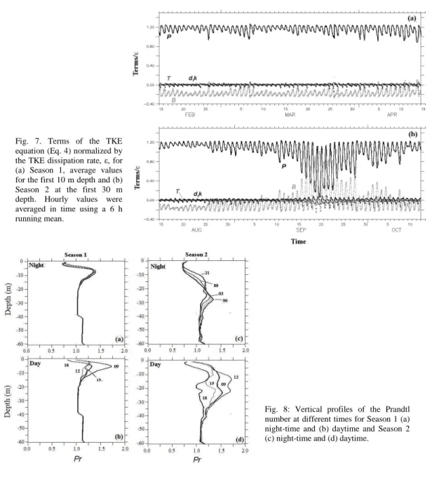
Figure 7 shows the terms of the TKE equation (Eq. 4) normalized by the dissipation rate (ε ) of TKE as described in Eq. 13, for each season, taking a depth of 10 m for Season 1 and 30 m for Season 2.
1 k T B
P t =
ε ∂ − +
+ (13)
The local variation of TKE (∂tk) and the
vertical diffusion of TKE (T) are much smaller than the other terms. In Season 1, it may be observed that TKE is generated only by shear production (P) maintained by the surface wind stress in the shallow ML and that the buoyancy term (B) acts consuming TKE (negative values).
In Season 2 (Figure 7b) it is shown that, during some periods, the buoyancy term may act generating turbulence at night at the same rate as it produces shear during the day. This occurs due to the greater surface cooling at night in this season, promoting a statically unstable surface layer (convection).
Figures 5b and 7b show that during September 15 - 25, there is a deepening of the ML due to convection, as a result of the fact that during this period considerable buoyancy is produced at night. In the daytime, the buoyancy term acts to consume TKE, generated by the solar radiation, thus inducing a re-stratification of the ML. In Season 1 the stratified state of the upper layer prevents the production of turbulent buoyancy and the energy provided mechanically, by the winds, is not enough to promote deep mixing.
The turbulent Prandtl number (Pr) provides the ratio of the turbulent viscosity to temperature diffusivity (Eq. 14). This parameter may provide an insight into what processes dominate the turbulent mixing in the flow, since the turbulent viscosity depends mainly on shear, while temperature diffusivity depends on thermal and then buoyancy effects. Therefore, regions where Pr > 1 signifies a predominance of the mechanical production of TKE (Eq. 5) and where Pr < 1, a predominance of the buoyancy production of TKE (Eq. 6).
h t m
t ν
ν /
Pr= (14)
Figure 8 compares the vertical profile of the Prandtl number (Pr) for each season averaged at different hours. In Season 1 after 18 h (Fig. 8) the Pr diminishes at the surface and then, at night (Fig. 8a), the turbulent diffusivity of temperature (νth) is
dominant at the first 5 m depth. This fact shows the influence of the nocturnal turbulent cooling that, despite the low values, is responsible for a deepening of the ML at night. The turbulent viscosity (νtm)
dominates rapidly at depths greater than around 20 m.
Below this depth, both coefficients are of the same order. During daytime (Figure 8b), the turbulent viscosity is dominant in the ML (Pr > 1). A step-like change is observed in the Prandtl number at around 40 m depth with values greater than one, both during night (Fig. 8a) and the day (Fig. 8b), probably associated with the increase in the shear caused by the presence of the EUC near this depth. According to Figure 3, the core of the EUC varies, during Season 1, from 50 to 80 m.
The νth is dominant over a great part of the
ML at night during Season 2 (Fig. 8c), characterizing a
period of convective turbulence production. From 18 h (Figure 8d) to 06 h (Fig. 8c) a progressive increase of νt
h
over νt m
is verified, the former being comparatively greater around 15 m, from 03 to 06 h. Below this depth, turbulent viscosity dominates as far as the region of EUC influence (eastward flow, from around 30 m deep, Fig. 4b). During daytime the temperature turbulent viscosity dominates. From 09 h to 12 h there is an increase in the νtm and a reduction of the νth,
which can be related to an increase in the shear production (Fig. 7b). After 12 h the νtm values
decrease.
Fig. 7. Terms of the TKE equation (Eq. 4) normalized by the TKE dissipation rate, ε, for (a) Season 1, average values for the first 10 m depth and (b) Season 2 at the first 30 m depth. Hourly values were averaged in time using a 6 h running mean.
D
ISCUSSIONIn this study the second-order turbulent closure of Canuto et al. (2001) using the k-ε equations version of the General Ocean Turbulence Model (GOTM, Burchard et al., 1999) was applied over the equatorial Atlantic region to investigate the main features of the mixing layer of two well defined seasons in respect of the atmospheric forcing and the state of the upper ocean. The former occurs in the presence of the intertropical convergence zone – identified as Season 1 - and the latter when the ITCZ is displaced northwards – identified as Season 2.
To compute the surface flux boundary conditions, the PIRATA dataset from the buoy located at 0o lat., 23o W was used, using the algorithm of the Coupled Ocean-Atmosphere Response Experiment (Fairall et al., 2003). The PIRATA dataset was also used in the procedure of data assimilation during the numerical simulation of the water column´s mean properties. Complementarily, the radiation dataset from NASA/GEWEX Surface Radiation Budget Project was used to close the surface radiation balance. The surface fluxes presented only a small annual cycle despite the variability of the sea surface temperature occurring on this time scale. The slightly higher net surface heat was found during Season 1 due mainly to the lesser wind-induced latent heat lost.
The assimilation scheme used in this project reproduced the main features of the equatorial region faithfully, permitting a realistic representation of the turbulent properties and therefore allowing a comparison between the ML in the two seasons.
The estimated ML depth values are in agreement with the climatological estimate of Monterey and Levitus (1997) and Montegut el al. (2004). In Season 1, the maximum depth reached by the simulated ML was 15 m, showing an averaged diurnal variation of 7 m, while in Season 2, the ML depth reached approximately 60 m with an averaged diurnal variability of about 30 m.
The analysis of the heat accumulated at the surface, obtained from the computed surface heat fluxes, and of the accumulated heat at different water column depths, obtained from the assimilated temperature vertical profile, showed the differences in the ML heat content in each season, as previously described by the observational work of Weisberg and Weingartner (1999a,b). The results showed that the ML heat accumulated during Season 1 is not in equilibrium with the surface net heat probably due to the temperature advection during this period, while in Season 2 a certain balance was verified (Figure 6).
The simulations indicated that the production of turbulent kinetic energy in the ML varies seasonally over the Tropical Atlantic. In Season 1, the low wind intensity at the surface provides a
small mechanical production of TKE. Besides, the highly stable stratification of the upper layer acts in such a way as to consume significant fractions of the TKE in the ML. Thus both effects prevent the growth of the ML during Season 1. On the other hand, the intensification of the wind velocity in Season 2 increases the mechanical production of TKE in the ML. Thermal convection induced by nocturnal surface cooling contributes to an increase in the TKE, promoting a deepening of the ML during Season 2.
Analyses of the Prandtl number at different times during each season showed that in Season 2, during night-time, the estimated temperature turbulent diffusivity is more important at the first 15 m depth than the turbulent viscosity, suggesting the existence of a convective regime of the nocturnal ML, probably caused by the increase in the surface longwave net lost. The convection observed at night and the re-stratification and suppression of TKE by the buoyancy term appears to be responsible for the higher amplitude of the diurnal variation of the depth of the ML during this season.
A
CKNOWLEDGEMENTSThis work was financed by CNPq and Fapesp.
R
EFERENCESBOLDING, K.; BURCHARD, H.; POHLMANN, T.; STIPS, A. Turbulent mixing in the Northern North Sea: a numerical model study. Cont. Shelf Res., v. 22, 2002. p. 2707-2724.
BOURLÈS, B.; MCPAHADEN, M. J.; HERNANDES, F.; NOBRE, P.; CAMPOS, E.; YU, L.; PLANTON, S.; BUSALACCHI, A., MOURA, A. D.; SERVAIN, J.; TROTTE, J. The PIRATA Program. History, accomplishments, and future directions. Bull. Amer.
Meteor. Soc., 2008. p. 1111-1125,
DOI:10.1175/2008BAMS2462.1.
BURCHARD, H.; BAUMERT, H. On the performance of a mixed-layer model based on the k-epsilon turbulence closure. J. Geophys. Res., v. 100, 1995. p. 8523-8540. BURCHARD, H.; BOLDING, K. Comparative analysis of
four second-moment turbulence closure models for the oceanic mixed layer. J. Phys. Oceanogr., v. 31, 2001. p. 1943-1968.
BURCHARD, H.; BOLDING, K.; VILLARREAL, M. GOTM – a general ocean turbulence model. Theory, applications and test cases. Tech.Rep. EUR 18745 EN, European Commission.
CANUTO, V. M.; HOWARD, A.; CHENG, Y.; DUBOVIKOV, M. S. Ocean turbulence. Part I: One point closure model, momentum and heat vertical diffusivities. J. Phys. Oceanogr., v. 31 (6), 2001. p. 1413-1426.
CARTON, J. A.; ZHOU, Z. Annual cycle of sea surface temperature in the tropical Atlantic Ocean. J. Geophy.
Res., v. 102, 1997. p. 27813-27824.
CHANG, P.; SARAVANAN, L.; JI, L.; HEGERL, G.C. The effect of local sea surface temperatures on atmospheric circulation over the tropical Atlantic sector. J. Climate, v. 13, 2000. p. 2195-2216.
DE BOYER MONTÉGUTE C.; MADEC, G.; FISHER, A. S.; LASAR, A.; IUDICONE, D. Mixed layer depth over the global ocean: an examination of profile data and a profile-based climatology. J. Geophys. Res., v. 109, 2004. DOI:10.1029/2004JC002378.
FAIRALL, C. W.; BRADLEY, E. F.; HARE, J. E.; GRACHEV, A. A.; EDSON, J. B. Bulk Parameterization of Air-Sea Fluxes: Updates and Verification for the COARE Algorithm. J. of Climate, v. 16, 2003. p. 571-591.
HASTENRATH, S. Climate Dynamics of the Tropics. Kluwer Academic, 1991. 488p.
JEFREY, C. D.; ROBINSON, I. S.; WOOLF, D. K.; DONLON, C. J. The response to phase-dependent wind stress and cloud fraction of the diurnal cycle of SST and air–sea CO2 exchange. Ocean Modelling. v. 23, 2008. p. 33-48.
LEVITUS, S.; BOYER, T. P. Temperature. World Ocean
Atlas 1994. NOAA Atlas NESDIS 4. v. 4, 1994. 117p.
MOISAN, J.; NIILER, P. The seasonal heat budget of the North Pacific: net heat fluxes and heat storage rates (1950-90). J. Phys. Oceanogr. v. 28, 1998. p. 401-421. MONTEREY, G.; LEVITUS, S. Seasonal Variability of
Mixed Layer Depth for the World Ocean. NOAA
Atlas NESDIS 14, Natl. Oceanic and Atmos. Admin., Silver Spring, Md. 5 p.
PERES, J. R. 2008. Estudo do balanço de radiação sobre o oceano Atlântico Tropical na região do Arquipélago de São Pedro e São Paulo. Relatório Final de Iniciação Científica. Instituto de Astronomia, Geofísica e Ciências Atmosféricas. Universidade de São Paulo. 2008. 35 p. http://www.iag.usp.br/meteo/labmicro/publicacoes/relato rios_tecnicos/Jean_2008_Estudo_do_balanco_de_radiac ao_sobre_o_oceano_Atlantico_tropical_na_regiao_do_A SPSP.pdf
PHILANDER, S. G. El Niño, La Niña, and Southern
Oscillation. Academic Press, Londres, 289. 1990. 289 p.
WEINGARTNER, T. J.; WEISBERG, R. H. On the annual cycle of equatorial upwelling in the central Atlantic Ocean. J. Phys. Oceanogr. v. 21, 1991a. p. 68-82. WEINGARTNER, T. J.; WEISBERG, R. H. A description of
the annual cycle in the sea surface temperature and upper ocean heat in the equatorial Atlantic. J. Phys. Oceanogr. v. 21, 1991b. p. 82-96.
WEISBERG, T. J.; TANG, T. Y. Further studies on the response of the equatorial thermocline in the Atlantic Ocean to the seasonal varying trade winds. J. Phys.
Oceanogr. v. 92, 1987. p. 3709-3727.
YU, L.; XIANGZE, X.; WELLER, R. A. Role of net surface heat fluxes in seasonal variations of sea surface temperature in the tropical Atlantic Ocean. J. Climate. v. 19, 2006. p. 6153-6169.
YU, L.; XIANGZE, X.; WELLER, R. A. Multidecade
Global Flux Datasets from the Objectively Analyzed Air-sea Fluxes (OAFlux) Project: Latent and Sensible Heat Fluxes, Ocean Evaporation, and Related Surface Meteorological Variables. Woods Hole
Oceanographic Institution. OAFlux Project Technical Report, 2008. 64p.
ZHANG, Y. C.; ROSSOW, W. B.; LACIS, A. A.; OINAS, V.; MISHCHENKO, M. I. Calculation of radiative fluxes from the surface to top of atmosphere based on ISCCP and other global data sets: refinements of the radiative transfer model and input data. J. Geophys. Res. v. 109, D19105, 2004. DOI: 10.1029/2003JD004457.